
Panel Data Analysis
Fixed and Random Effects
using Stata
(v. 6.0)
Oscar Torres-Reyna
otorres@princeton.edu
December 2007 http://www.princeton.edu/~otorres/

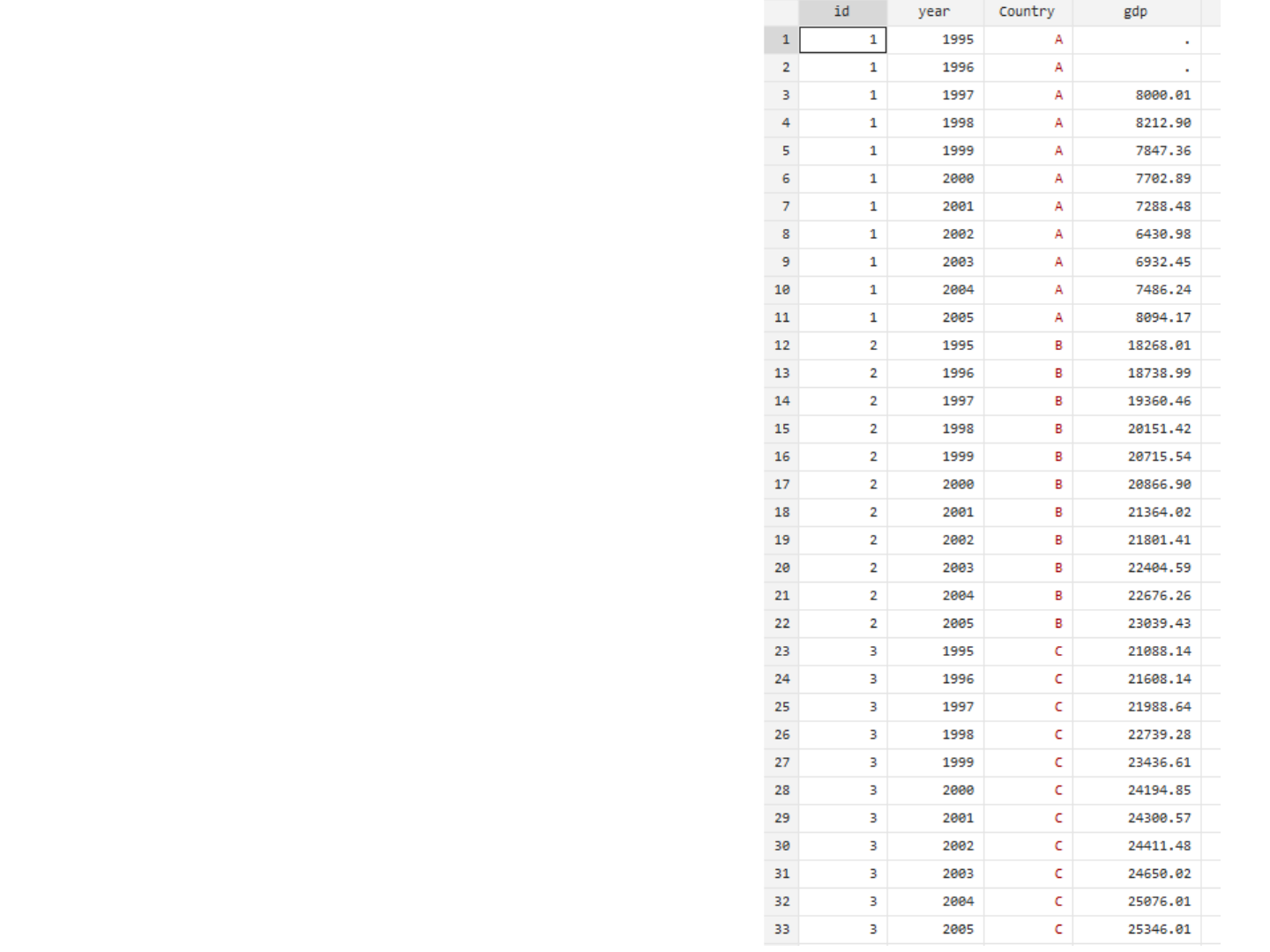
What panel data looks like…
Panel data (also known as
longitudinal or cross-
sectional time-series data)
is a dataset in which the
behavior of entities (i) are
observed across time (t).
(X
it
, Y
it
), i=1,…n; t=1,…T
These entities could be
states, companies, families,
individuals, countries, etc.
See Stock and Watson, Introduction to Econometrics, chapter 10 “Regression with Panel Data”.
OTR 2
Entity
Year Y X1 X2 X3 …..
1 1 # # # # …..
1 2 # # # # …..
1 3 # # # # …..
: : : : : : :
2 1 # # # # …..
2 2 # # # # …..
2 3 # # # # …..
: : : : : : :
3 1 # # # # …..
3 2 # # # # …..
3 3 # # # # …..

Preparing Data into Panel
Data format
OTR 3

The data: the long form
To analyze panel data:
• Variables should be in
columns.
• Entity and time in
rows.
This format is known as
long form.
OTR 4
Entity
Year Y X1 X2 X3 …..
1 1 # # # # …..
1 2 # # # # …..
1 3 # # # # …..
: : : : : : :
2 1 # # # # …..
2 2 # # # # …..
2 3 # # # # …..
: : : : : : :
3 1 # # # # …..
3 2 # # # # …..
3 3 # # # # …..

Wide form data (time in columns)
If your dataset is in wide format, either entity or time
are in columns, you need to reshape it to long format
(you can do this in Stata).
Beware that Stata does not like numbers as column
names. You need to add a letter to the numbers
before importing into Stata. If you have something
like the following:
OTR 5

Wide form data (time in columns)
Add a letter to the numeric column names, for example,
an ‘x’ before the year:
OTR 6
Import into Stata
Reshaping from wide to
long
Once in Stata, you can reshape
it using the command
reshape:
OTR 7
gen id = _n
order id
reshape long x , i(id) j(year)
rename x gdp
Type help reshape for more details

Wide form data (entity in columns)
If the wide format data has the entities in column
and time in rows, like this example:
OTR 8

Wide form data (entity in columns)
Import it into Stata:
OTR 9

Reshape wide to long format
Once in Stata, you can reshape it
using the command reshape:
OTR 10
* Adding the prefix ‘gdp’ to column names.
Command ‘renvars’ is user-written, you need
to install it, see note below
renvars A-G, pref(gdp)
gen id = _n
order id
reshape long gdp , i(id) j(country) str
Type help reshape for more details.
You need to install renvars, type:
search renvars
Click on the link for dm88_* then install.

More than one variable in same column
To reshape data from wide to long where more than one variable is in the same
column like the example below, see slides 29 to 32 in this document:
https://www.princeton.edu/~otorres/DataPrep101.pdf#page=29
OTR 11
If you are downloading data from the World Development Indicators, see slide
21 in the link below to get it in the proper panel data form without the need to
reshape: https://www.princeton.edu/~otorres/FindingData101.pdf#page=21
Entity Year Variable Value
A 1 Var1 ###
A 2 Var1 ###
A 3 Var1 ###
A 1 Var2 ###
A 2 Var2 ###
A 3 Var2 ###
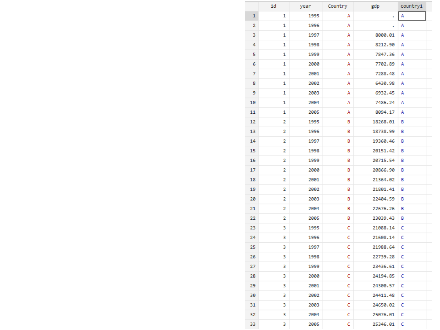
Assign numbers to strings
The encode command assigns
a number to the string variable
in alphabetical order.
The new variable is a labeled
variable where the labels are
the original strings assigned to
specific number.
Notice that string variables
have the color red, while
labeled variables have color
blue.
Type help encode for more
info.
OTR 12

Setting data as panel
Once the data is in long form, we need to set it as panel so we can
use Stata’s panel data xt commands and the time series operators.
Using the example from the previous page type:
xtset country year
string variables not allowed in varlist;
Country is a string variable
Given the error, we need to have ‘country’ in numeric format.
Type
encode country, gen(country1)
Then using ‘country1’ type
xtset country1 year
Panel variable: country1 (strongly balanced)
Time variable: year, 2000 to 2021
Delta: 1 unit
OTR 13
Balanced panel: all entities are
observed across all times.
Unbalanced panel: some entities
are not observed in some years.
Stata algorithms automatically
account for this.

Visualizing panel data
Once the data is set as panel, you can use a series of xt commands
to analyze it. For more information type:
help xt
A useful visualization command is xtline, type:
xtline gdp
OTR 14

Visualizing panel data
* All in one, type:
xtline gdp, overlay
OTR 15

Usage
Panel data deals with omitted variable bias due to heterogeneity in
the data. It does this by controlling for variables that we cannot
observe, are not available, and/or can not be measured but are
correlated with the predictors. Two types:
1. Variables that do not change over time but vary across entities
(cultural factors, difference in business practices across
companies, etc.) → Entity fixed effects.
2. Variables that change over time but not across entities (i.e.
national policies, federal regulations, international
agreements, etc.) → Time fixed effects.
Some drawbacks when working with panel data are data collection
issues (i.e. sampling design, coverage), non-response in the case of
micro panels or cross-country dependency in the case of macro
panels (i.e. correlation between countries).
OTR 16
For a comprehensive list of advantages and disadvantages of panel data see Baltagi, Econometric
Analysis of Panel Data (chapter 1).

FIXED-EFFECTS MODEL
(Covariance Model, Within
Estimator, Individual Dummy
Variable Model, Least Squares
Dummy Variable Model)
OTR 17

The fixed effects idea
Entities have individual characteristics that may
or may not influence the outcome and/or
predictor variables. For example, the business
practices of a company may influence its stock
price or level of spending; attitudes or policies
towards guns in a particular state may affect its
levels of gun violence. Business practices,
cultural, or political variables are, most of the
time unavailable or hard to measure.
OTR 18

The fixed effects idea
Since individual characteristics are not random
and may impact the predictor or outcome
variables, we need to control for them. In this
way, the effect of the predictors will not be
influenced by those fixed characteristics.*
In entity’s fixed effects it is assumed a
correlation between the entity’s error term and
predictor variables. However, an entity’s fixed
effects cannot be correlated with another
entity’s.
OTR 19
* See Stock and Watson, 2003, p.289-290

The model (1)
The entity fixed effects regression model is
i = 1…n ; t = 1….T
Where:
outcome variable (for entity i at time t).
is the unknown intercept for each entity (n entity-specific intercepts).
is a vector of predictors (for entity i at time t) .
within-entity error term ;
overall error term.
Interpretation of the coefficient: for a given entity, when a
predictor changes one unit over time, the outcome will
increase/decrease by units (assuming no transformation is
applied).* Here, represents a common effect across entities
controlling for individual heterogeneity.
OTR 20
* See Bartels, Brandom, “Beyond “Fixed Versus Random Effects”: A framework for improving substantive and statistical
analysis of panel, time-series cross-sectional, and multilevel data”, Stony Brook University, working paper, 2008

The model (2)
The entity and time fixed effects regression model is
i = 1…n ; t = 1….T
Where:
outcome variable (for entity i at time t).
is the unknown intercept for each entity (n entity-specific intercepts).
is a vector of predictors (for entity i at time t) .
is the unknow coefficient for the time regressors (t)
within-entity error term ;
overall error term.
Interpretation of a coefficient: for a given entity, when a
predictor changes one unit over time, the outcome will
increase/decrease by units (assuming no transformation is
applied).* Here, represents a common effect across entities
controlling for individual and time heterogeneity.
OTR 21
* See Bartels, Brandom, “Beyond “Fixed Versus Random Effects”: A framework for improving substantive and statistical
analysis of panel, time-series cross-sectional, and multilevel data”, Stony Brook University, working paper, 2008

Data example
The data used in the following slides was extracted from the World
Development Indicators database:
https://databank.worldbank.org/source/world-development-indicators
Selected variables since 2000, all countries only:
• GDP per capita (constant 2015 US$)
• Exports of goods and services (constant 2015 US$)
• Imports of goods and services (constant 2015 US$)
• Labor force, total
Data was further cleaned to remove regions, subregions, and missing values
across years and variables resulting in 126 countries.
Variable ‘trade’ was added by adding imports + exports.
OTR 22

Setting data as panel
Once the data is in long form, we need to set it as panel so we can
use Stata’s panel data xt commands and the time series operators.
Using the example from the previous page type:
xtset country year
string variables not allowed in varlist;
Country is a string variable
Given the error, we need to have ‘country’ in numeric format.
Type
encode country, gen(country1)
Then using ‘country1’ type
xtset country1 year
Panel variable: country1 (strongly balanced)
Time variable: year, 2000 to 2021
Delta: 1 unit
OTR 23
Balanced panel: all entities are
observed across all times.
Unbalanced panel: some entities
are not observed in some years.
Stata algorithms automatically
account for this.

* Not ideal with many panels
xtline gdppc
OTR 24

* Getting the big picture
xtline gdppc, overlay legend(off)
OTR 25

* Heterogeneity across years
bysort year: egen mean_gdppc = mean(gdppc)
twoway scatter gdppc year, msymbol(circle_hollow) color(gs14) || ///
connected mean_gdppc year, msymbol(diamond) sort ///
ylabel(0(10000)115000, angle(0) labsize(2) format(%7.0fc)) ///
xlabel(2000(1)2021, angle(45) labsize(2) grid) ///
title(GDP per capita (constant 2015 US$)) xtitle(Year, size(2.5)) ///
legend(label(1 "GDPpc per country") label(2 "Mean GDPpc per year"))
OTR 26

Data example – transformations
To log-transformed a variable use the function ln():
gen ln_gdppc = ln(gdppc)
gen ln_labor = ln(labor)
gen ln_trade = ln(trade)
If the variable has negative values, you need to add a value high
enough so the minimum value is over zero (preferable 1). For
example, if the lowest value in ‘varX’ is -1, then type:
gen ln_varX = ln(varX + 2)
The natural log of 1 is zero.
OTR 27

Data example – histograms
OTR 28
hist gdppc
hist labor
hist trade

Data example – histograms
OTR 29
hist ln_gdppc
hist ln_labor
hist ln_trade

Descriptive statistics
. sum gdppc trade labor // Pooled data
Variable | Obs Mean Std. dev. Min Max
-------------+---------------------------------------------------------
gdppc | 2,772 14925.78 19561 261.0194 112417.9
trade | 2,772 2.39e+11 5.33e+11 1.28e+08 5.58e+12
labor | 2,772 1.70e+07 4.54e+07 85987 4.89e+08
. xtsum gdppc trade labor // Heterogeneity by panel and time
Variable | Mean Std. dev. Min Max | Observations
-----------------+--------------------------------------------+----------------
gdppc overall | 14925.78 19561 261.0194 112417.9 | N = 2772
between | 19404.61 293.4895 104003.7 | n = 126
within | 2991.204 -14918.74 52165.38 | T = 22
| |
trade overall | 2.39e+11 5.33e+11 1.28e+08 5.58e+12 | N = 2772
between | 5.20e+11 3.14e+08 4.33e+12 | n = 126
within | 1.27e+11 -1.14e+12 1.49e+12 | T = 22
| |
labor overall | 1.70e+07 4.54e+07 85987 4.89e+08 | N = 2772
between | 4.54e+07 132657 4.53e+08 | n = 126
within | 3154440 -4.24e+07 5.27e+07 | T = 22
OTR 30
See https://www.stata.com/manuals/xtxtsum.pdf

Fixed effects regression using xtreg, fe
OTR 31
. xtreg ln_gdppc ln_trade ln_labor, fe robust
Fixed-effects (within) regression Number of obs = 2,772
Group variable: country1 Number of groups = 126
R-squared: Obs per group:
Within = 0.6267 min = 22
Between = 0.3872 avg = 22.0
Overall = 0.3906 max = 22
F(2,125) = 87.57
corr(u_i, Xb) = 0.1067 Prob > F = 0.0000
(Std. err. adjusted for 126 clusters in country1)
------------------------------------------------------------------------------
| Robust
ln_gdppc | Coefficient std. err. t P>|t| [95% conf. interval]
-------------+----------------------------------------------------------------
ln_trade | .3603947 .0737076 4.89 0.000 .2145182 .5062712
ln_labor | .053167 .1608747 0.33 0.742 -.265224 .371558
_cons | -.9384681 1.075791 -0.87 0.385 -3.067592 1.190656
-------------+----------------------------------------------------------------
sigma_u | 1.1155513
sigma_e | .10989953
rho | .99038791 (fraction of variance due to u_i)
------------------------------------------------------------------------------
Outcome Predictor(s)
Fixed effects option
Controlling for
heteroskedasticity
Total number of
cases (rows)
Total number of entities (i)
If this number is < 0.05 then
your model is ok. This is an F-
test to see whether all the
coefficients in the model are
jointly different than zero.
Two-tail p-values test the
hypothesis that each coefficient is
different from 0 (according to its
t-value).
A value lower than 0.05 will reject
the null and conclude that the
predictor has a significant effect
on the outcome (95%
significance).
The within entity errors u
i
are correlated with the
regressors in the fixed
effects model.
Beta coefficients indicate the
change in the output (y) when
the predictors change one
unit over time. In this
example, all the variables are
log-transformed, the
interpretation is: when the
predictor increases 1% over
time, the output (y) changes
% (elasticity).
Intraclass correlation (rho), shows how much
of the variance in the output is explained by
the difference across entities. In this example
is 99%.
sigma_u = sd of residuals within groups
sigma_e = sd of residuals (overall error term)

Entity and time fixed effects regression using xtreg, fe
OTR 32
. xtreg ln_gdppc ln_trade ln_labor i.year, fe robust
Fixed-effects (within) regression Number of obs = 2,772
Group variable: country1 Number of groups = 126
R-squared: Obs per group:
Within = 0.7083 min = 22
Between = 0.7977 avg = 22.0
Overall = 0.7581 max = 22
F(23,125) = 34.28
corr(u_i, Xb) = 0.7525 Prob > F = 0.0000
(Std. err. adjusted for 126 clusters in country1)
------------------------------------------------------------------------------
| Robust
ln_gdppc | Coefficient std. err. t P>|t| [95% conf. interval]
-------------+----------------------------------------------------------------
ln_trade | .2401329 .0695213 3.45 0.001 .1025416 .3777242
ln_labor | -.2958837 .081081 -3.65 0.000 -.456353 -.1354145
|
year |
2001 | .0119809 .0042779 2.80 0.006 .0035144 .0204475
... ... ... ... ... ... ...
... ... ... ... ... ... ...
2021 | .2878247 .0705454 4.08 0.000 .1482065 .4274428
|
_cons | 7.213881 1.961627 3.68 0.000 3.331578 11.09619
-------------+----------------------------------------------------------------
sigma_u | 1.0561892
sigma_e | .09753735
rho | .99154389 (fraction of variance due to u_i)
------------------------------------------------------------------------------
Outcome Predictor(s)
Fixed effects option
Controlling for
heteroskedasticity
Total number of
cases (rows)
Total number of entities (i)
If this number is < 0.05 then
your model is ok. This is an F-
test to see whether all the
coefficients in the model are
jointly different than zero.
Two-tail p-values test the
hypothesis that each coefficient is
different from 0 (according to its
t-value).
A value lower than 0.05 will reject
the null and conclude that the
predictor has a significant effect
on the outcome (95%
significance).
The within entity errors u
i
are correlated with the
regressors in the fixed
effects model.
Beta coefficients indicate the
change in the output (y) when
the predictors change one
unit over time. In this
example, all the variables are
log-transformed, the
interpretation is: when the
predictor increases 1% over
time, the output (y) changes
% (elasticity).
Intraclass correlation (rho),
shows how much of the
variance in the output is
explained by the difference
across entities. In this
example is 99%.
sigma_u = sd of residuals within groups
sigma_e = sd of residuals (overall error term)
Time fixed effects

Fixed effects regression using xtreg, fe (with lags on predictors)
OTR 33
. xtreg ln_gdppc L1.ln_trade L1.ln_labor, fe robust
Fixed-effects (within) regression Number of obs = 2,646
Group variable: country1 Number of groups = 126
R-squared: Obs per group:
Within = 0.6054 min = 21
Between = 0.3771 avg = 21.0
Overall = 0.3799 max = 21
F(2,125) = 81.17
corr(u_i, Xb) = 0.1265 Prob > F = 0.0000
(Std. err. adjusted for 126 clusters in country1)
------------------------------------------------------------------------------
| Robust
ln_gdppc | Coefficient std. err. t P>|t| [95% conf. interval]
-------------+----------------------------------------------------------------
ln_trade |
L1. | .3385586 .0703993 4.81 0.000 .1992297 .4778875
|
ln_labor |
L1. | .0581167 .1566956 0.37 0.711 -.2520033 .3682367
|
_cons | -.4600892 1.082489 -0.43 0.672 -2.60247 1.682291
-------------+----------------------------------------------------------------
sigma_u | 1.1260807
sigma_e | .10685653
rho | .99107579 (fraction of variance due to u_i)
------------------------------------------------------------------------------
Outcome Predictor(s)
Fixed effects option
Controlling for
heteroskedasticity
Total number of
cases (rows)
Total number of entities (i)
If this number is < 0.05 then
your model is ok. This is an F-
test to see whether all the
coefficients in the model are
jointly different than zero.
Two-tail p-values test the
hypothesis that each coefficient is
different from 0 (according to its
t-value).
A value lower than 0.05 will reject
the null and conclude that the
predictor has a significant effect
on the outcome (95%
significance).
The within entity errors u
i
are correlated with the
regressors in the fixed
effects model.
Beta coefficients indicate
the change in the output
(y) when the predictors one
unit over time (a year
before –”L1.”). In this
example, all the variables
are log-transformed, the
interpretation is: when the
predictor increases 1% over
time (a year before –”L1.”),
the output (y) changes %
(elasticity).
Intraclass correlation (rho),
shows how much of the
variance in the output is
explained by the difference
across entities. In this
example is about 98%.
sigma_u = sd of residuals within groups
sigma_e = sd of residuals (overall error term)

Entity fixed effects regression using reghdfe
OTR 34
. reghdfe ln_gdppc ln_trade ln_labor , absorb(country1) vce(cluster country1)
(MWFE estimator converged in 1 iterations)
HDFE Linear regression Number of obs = 2,772
Absorbing 1 HDFE group F( 2, 125) = 87.57
Statistics robust to heteroskedasticity Prob > F = 0.0000
R-squared = 0.9943
Adj R-squared = 0.9940
Within R-sq. = 0.6267
Number of clusters (country1) = 126 Root MSE = 0.1099
(Std. err. adjusted for 126 clusters in country1)
------------------------------------------------------------------------------
| Robust
ln_gdppc | Coefficient std. err. t P>|t| [95% conf. interval]
-------------+----------------------------------------------------------------
ln_trade | .3603947 .0737076 4.89 0.000 .2145182 .5062712
ln_labor | .053167 .1608747 0.33 0.742 -.265224 .371558
_cons | -.9384681 1.075791 -0.87 0.385 -3.067592 1.190656
------------------------------------------------------------------------------
Absorbed degrees of freedom:
-----------------------------------------------------+
Absorbed FE | Categories - Redundant = Num. Coefs |
-------------+---------------------------------------|
country1 | 126 126 0 *|
-----------------------------------------------------+
* = FE nested within cluster; treated as redundant for DoF computation
Outcome Predictor(s)
Fixed effects option
Controlling for
correlation within
panels
Total number of
cases (rows)
Total number of entities (i)
If this number is < 0.05 then
your model is ok. This is an F-
test to see whether all the
coefficients in the model are
jointly different than zero.
Two-tail p-values test the
hypothesis that each coefficient is
different from 0 (according to its
t-value).
A value lower than 0.05 will reject
the null and conclude that the
predictor has a significant effect
on the outcome (95%
significance).
Beta coefficients indicate
the change in the output (y)
when the predictors change
one unit over time. In this
example, all the variables
are log-transformed, the
interpretation is: when the
predictor increases 1% over
time, the output (y) changes
% (elasticity).
R-squared shows the percent
of the variance in the outcome
explained by the model. The Adj
R-squared, accounts for the
number of variables and their
significant contribution to
explaining the variation in the
output variable.
NOTE: Use reghdfe when controlling for multiple fixed effects or when xtreg,fe cannot run due to the number
of panels.
Entity and time fixed effects regression using reghdfe
OTR 35
. reghdfe ln_gdppc ln_trade ln_labor , absorb(country1 year) vce(cluster country1)
(MWFE estimator converged in 2 iterations)
HDFE Linear regression Number of obs = 2,772
Absorbing 2 HDFE groups F( 2, 125) = 11.37
Statistics robust to heteroskedasticity Prob > F = 0.0000
R-squared = 0.9955
Adj R-squared = 0.9953
Within R-sq. = 0.3050
Number of clusters (country1) = 126 Root MSE = 0.0976
(Std. err. adjusted for 126 clusters in country1)
------------------------------------------------------------------------------
| Robust
ln_gdppc | Coefficient std. err. t P>|t| [95% conf. interval]
-------------+----------------------------------------------------------------
ln_trade | .2401329 .0695213 3.45 0.001 .1025416 .3777242
ln_labor | -.2958837 .081081 -3.65 0.000 -.456353 -.1354145
_cons | 7.381277 1.999695 3.69 0.000 3.423632 11.33892
------------------------------------------------------------------------------
Absorbed degrees of freedom:
-----------------------------------------------------+
Absorbed FE | Categories - Redundant = Num. Coefs |
-------------+---------------------------------------|
country1 | 126 126 0 *|
year | 22 0 22 |
-----------------------------------------------------+
* = FE nested within cluster; treated as redundant for DoF computation
Outcome Predictor(s)
Fixed effects option
Controlling for
correlation within
panels
Total number of
cases (rows)
Total number of entities (i)
If this number is < 0.05 then
your model is ok. This is an F-
test to see whether all the
coefficients in the model are
jointly different than zero.
Two-tail p-values test the
hypothesis that each coefficient is
different from 0 (according to its
t-value).
A value lower than 0.05 will reject
the null and conclude that the
predictor has a significant effect
on the outcome (95%
significance).
Beta coefficients indicate
the change in the output (y)
when the predictors change
one unit over time. In this
example, all the variables
are log-transformed, the
interpretation is: when the
predictor increases 1% over
time, the output (y) changes
% (elasticity).
R-squared shows the percent
of the variance in the outcome
explained by the model. The Adj
R-squared, accounts for the
number of variables and their
significant contribution to
explaining the variation in the
output variable.

Entity fixed effects regression with lags using reghdfe
OTR 36
reghdfe ln_gdppc L1.ln_trade L1.ln_labor , absorb(country1 ) vce(cluster country1)
(MWFE estimator converged in 1 iterations)
HDFE Linear regression Number of obs = 2,646
Absorbing 1 HDFE group F( 2, 125) = 81.17
Statistics robust to heteroskedasticity Prob > F = 0.0000
R-squared = 0.9946
Adj R-squared = 0.9943
Within R-sq. = 0.6054
Number of clusters (country1) = 126 Root MSE = 0.1069
(Std. err. adjusted for 126 clusters in country1)
------------------------------------------------------------------------------
| Robust
ln_gdppc | Coefficient std. err. t P>|t| [95% conf. interval]
-------------+----------------------------------------------------------------
ln_trade |
L1. | .3385586 .0703993 4.81 0.000 .1992297 .4778875
|
ln_labor |
L1. | .0581167 .1566956 0.37 0.711 -.2520033 .3682367
|
_cons | -.4600892 1.082489 -0.43 0.672 -2.60247 1.682291
------------------------------------------------------------------------------
Absorbed degrees of freedom:
-----------------------------------------------------+
Absorbed FE | Categories - Redundant = Num. Coefs |
-------------+---------------------------------------|
country1 | 126 126 0 *|
-----------------------------------------------------+
* = FE nested within cluster; treated as redundant for DoF computation
Outcome Predictor(s)
Fixed effects option
Controlling for
correlation within
panels
Total number of
cases (rows)
Total number of entities (i)
If this number is < 0.05 then
your model is ok. This is an F-
test to see whether all the
coefficients in the model are
jointly different than zero.
Two-tail p-values test the
hypothesis that each coefficient is
different from 0 (according to its
t-value).
A value lower than 0.05 will reject
the null and conclude that the
predictor has a significant effect
on the outcome (95%
significance).
Beta coefficients indicate
the change in the output (y)
when the predictors change
one unit over time. In this
example, all the variables
are log-transformed, the
interpretation is: when the
predictor increases 1% over
time, the output (y) changes
% (elasticity).
R-squared shows the percent
of the variance in the outcome
explained by the model. The Adj
R-squared, accounts for the
number of variables and their
significant contribution to
explaining the variation in the
output variable.
NOTE: must type xtset country1 year, before using lags in reghdfe

A note on fixed effects
“...The fixed-effects model controls for all time-invariant
differences between the individuals, so the estimated coefficients
of the fixed-effects models cannot be biased because of omitted
time-invariant characteristics...[like culture, religion, gender, race,
etc].
One side effect of the features of fixed-effects models is that they
cannot be used to investigate time-invariant causes of the
dependent variables. Technically, time-invariant characteristics of
the individuals are perfectly collinear with the person [or entity]
dummies. Substantively, fixed-effects models are designed to
study the causes of changes within a person [or entity]. A time-
invariant characteristic cannot cause such a change, because it is
constant for each person.” [(Underline is mine) Kohler, Ulrich,
Frauke Kreuter, Data Analysis Using Stata, 2
nd
ed., p.245]
OTR 37

RANDOM-EFFECTS MODEL
(Random Intercept, Partial
Pooling Model)
OTR 38

The random effects idea
The rationale behind random effects model is that, unlike the
fixed effects model, the variation across entities is assumed
to be random and uncorrelated with the predictor or
independent variables included in the model:
“...the crucial distinction between fixed and random effects is
whether the unobserved individual effect embodies elements that
are correlated with the regressors in the model, not whether these
effects are stochastic or not” [Green, 2008, p.183]
If you have reason to believe that differences across entities
have some influence on your dependent variable but are not
correlated with the predictors then you should use random
effects. An advantage of random effects is that you can
include time invariant variables (i.e. gender). In the fixed
effects model these variables are absorbed by the intercept.
OTR 39
Thanks to Mateus Dias for useful feedback.

The random effects idea
Random effects assume that the entity’s error term is not
correlated with the predictors which allows for time-
invariant variables to play a role as explanatory variables.
In random-effects you need to specify those individual
characteristics that may or may not influence the
predictor variables. The problem with this is that some
variables may not be available therefore leading to
omitted variable bias in the model.
RE allows to generalize the inferences beyond the sample
used in the model.
OTR 40

Random effects regression using xtreg, re
OTR 41
. xtreg ln_gdppc ln_trade ln_labor, re robust
Random-effects GLS regression Number of obs = 2,772
Group variable: country1 Number of groups = 126
R-squared: Obs per group:
Within = 0.6110 min = 22
Between = 0.7295 avg = 22.0
Overall = 0.7212 max = 22
Wald chi2(2) = 192.71
corr(u_i, X) = 0 (assumed) Prob > chi2 = 0.0000
(Std. err. adjusted for 126 clusters in country1)
------------------------------------------------------------------------------
| Robust
ln_gdppc | Coefficient std. err. z P>|z| [95% conf. interval]
-------------+----------------------------------------------------------------
ln_trade | .4175909 .0760404 5.49 0.000 .2685543 .5666274
ln_labor | -.1597685 .1312262 -1.22 0.223 -.4169671 .0974302
_cons | .9295612 .6361615 1.46 0.144 -.3172923 2.176415
-------------+----------------------------------------------------------------
sigma_u | .41594682
sigma_e | .10989953
rho | .93474564 (fraction of variance due to u_i)
------------------------------------------------------------------------------
Outcome Predictor(s)
Random effects option
Controlling for
heteroskedasticity
Total number of
cases (rows)
Total number of entities (i)
If this number is < 0.05 then
your model is ok. This is an F-
test to see whether all the
coefficients in the model are
jointly different than zero.
Two-tail p-values test the
hypothesis that each coefficient is
different from 0 (according to its
t-value).
A value lower than 0.05 will reject
the null and conclude that the
predictor has a significant effect
on the outcome (95%
significance).
The between entity errors
u
it
are uncorrelated with
the regressors in the
random effects model.
Beta coefficients indicate the
change in the output (y) when
the predictors change one
unit over time and across
entities (average effect). In
this example, all the variables
are log-transformed, the
interpretation is: when the
predictor increases, on
average, 1%, the output (y)
changes % (elasticity).
Intraclass correlation (rho), shows how much
of the variance in the output is explained by
the difference across entities. In this example
is 99%.
sigma_u = sd of residuals within groups
sigma_e = sd of residuals (overall error term)

FIXED OR RANDOM?
OTR 42

Which to choose?
Whenever there is a clear idea that individual characteristics of
each entity or group affect the regressors, use fixed effects. For
example, macroeconomic data collected for most countries
overtime. There might be a good reason to believe that
countries’ economic performance may be affected by their
own internal characteristics: type of government, political
environment, cultural characteristics, type of public policies,
etc.
Random effects is used whenever there is reason to believe
that individual characteristics have no effect on the regressors
(uncorrelated).
OTR 43

Which to choose?
The Hausman-test tests whether the individual characteristics are correlated with the regressors
(see Green, 2008, chapter 9). The null hypothesis is that they are not (random effects).
xtreg ln_gdppc ln_trade ln_labor, fe
estimates store fixed
xtreg ln_gdppc ln_trade ln_labor, re
estimates store random
hausman fixed random, sigmamore
. hausman fixed random, sigmamore
---- Coefficients ----
| (b) (B) (b-B) sqrt(diag(V_b-V_B))
| fixed random Difference Std. err.
-------------+----------------------------------------------------------------
ln_trade | .3603947 .4175909 -.0571962 .0026039
ln_labor | .053167 -.1597685 .2129354 .012825
------------------------------------------------------------------------------
b = Consistent under H0 and Ha; obtained from xtreg.
B = Inconsistent under Ha, efficient under H0; obtained from xtreg.
Test of H0: Difference in coefficients not systematic
chi2(2) = (b-B)'[(V_b-V_B)^(-1)](b-B)
= 484.43
Prob > chi2 = 0.0000
OTR 44
If Prob > chi2 is < 0.05 use fixed effects

TESTS / DIAGNOSTICS
OTR 45

Do we need time fixed effects?
To see if time fixed effects are needed when running a FE model use
the command testparm. It is a joint F-test to if all years jointly
equal to 0 (type help testparm for more details).
xtreg ln_gdppc ln_trade ln_labor i.year, fe robust
testparm i.year
OTR 46
. testparm i.year
( 1) 2001.year = 0
( 2) 2002.year = 0
( 3) 2003.year = 0
( 4) 2004.year = 0
( 5) 2005.year = 0
( 6) 2006.year = 0
( 7) 2007.year = 0
( 8) 2008.year = 0
( 9) 2009.year = 0
(10) 2010.year = 0
(11) 2011.year = 0
(12) 2012.year = 0
(13) 2013.year = 0
(14) 2014.year = 0
(15) 2015.year = 0
(16) 2016.year = 0
(17) 2017.year = 0
(18) 2018.year = 0
(19) 2019.year = 0
(20) 2020.year = 0
(21) 2021.year = 0
F( 21, 125) = 4.44
Prob > F = 0.0000
The Prob > F is < 0.05, we fail to
accept the null that the coefficients for
the years are jointly equal to zero. In this
case, time fixed effects are needed.

Do we need random effects?
The LM test helps you decide between a random effects regression
and a simple OLS regression. The null hypothesis in the LM test is
that variances across entities is equal to zero. This is, no significant
difference across units (i.e. no panel effect). The command in Stata
is xttset0 type it right after running the random effects model
xtreg ln_gdppc ln_trade ln_labor, re robust
xttest0
. xttest0
Breusch and Pagan Lagrangian multiplier test for random effects
ln_gdppc[country1,t] = Xb + u[country1] + e[country1,t]
Estimated results:
| Var SD = sqrt(Var)
---------+-----------------------------
ln_gdppc | 2.022383 1.422105
e | .0120779 .1098995
u | .1730118 .4159468
Test: Var(u) = 0
chibar2(01) = 19981.51
Prob > chibar2 = 0.0000
OTR 47
Prob > chibar2 < 0.05, we fail to
accept the null hypothesis and conclude
that random effects are needed.

Are the panels correlated? [B-P/LM test]
According to Baltagi, cross-sectional dependence is a problem in macro panels
with long time series (over 20-30 years). The null hypothesis in the B-P/LM test of
independence is that residuals across entities are not correlated. The user-
defined command to run this test is xttest2 (run it after xtreg, fe):
ssc install xttest2
xtreg ln_gdppc ln_trade ln_labor, fe robust
xttest2
. xttest2
Correlation matrix of residuals:
[OMITTED]
Breusch-Pagan LM test of independence: chi2(7875) = 73886.228, Pr = 0.0000
Based on 22 complete observations over panel units
OTR 48
Pr < 0.05, we fail to accept the null hypothesis and conclude that panel are
correlated (cross-sectional dependence).

Are the panels correlated? [Pasaran CD test]
As mentioned in the previous slide, cross-sectional dependence is more of an issue in macro panels
with long time series (over 20-30 years) than in micro panels.
Pasaran CD (cross-sectional dependence) test is used to test whether the residuals are
correlated across entities*. Cross-sectional dependence can lead to bias in tests results (also called
contemporaneous correlation). The null hypothesis is that residuals are not correlated. The command
for the test is xtcsd, you have to install it typing:
ssc install xtcsd
xtreg ln_gdppc ln_trade ln_labor, fe robust
xtcsd, pesaran abs
. xtcsd, pesaran abs
Pesaran's test of cross sectional independence = 9.266, Pr = 0.0000
Average absolute value of the off-diagonal elements = 0.588
OTR 49
Pr < 0.05, we fail to accept the null
hypothesis and conclude that panel
are correlated (cross-sectional
dependence).
Had cross-sectional dependence be present Hoechle suggests to use Driscoll and Kraay standard errors
using the command xtscc (install it by typing ssc install xtscc). Type help xtscc for more
details.
*Source: Hoechle, Daniel, “Robust Standard Errors for Panel Regressions with Cross-Sectional Dependence”,
http://fmwww.bc.edu/repec/bocode/x/xtscc_paper.pdf

Testing for heteroskedasticity
A test for heteroskedasticity is available for the fixed- effects model using the
command xttest3. The null hypothesis is homoskedasticity (or constant
variance). This is a user-written program, to install it type:
ssc install xttest3
xtreg ln_gdppc ln_trade ln_labor, fe robust
xttest3
. xttest3
Modified Wald test for groupwise heteroskedasticity
in fixed effect regression model
H0: sigma(i)^2 = sigma^2 for all i
chi2 (126) = 3.3e+05
Prob>chi2 = 0.0000
OTR 50
We reject the null and conclude
heteroskedasticity.
NOTE: Use the option ‘robust’ to obtain heteroskedasticity-robust standard errors (also known
as Huber/White or sandwich estimators).

Testing for serial correlation
Serial correlation tests apply to macro panels with long time series (over 20-30 years).
Not a problem in micro panels (with very few years). Serial correlation causes the
standard errors of the coefficients to be smaller than they actually are and higher R-
squared. A Lagram-Multiplier test for serial correlation is available using the command
xtserial. This is a user-written program, to install it type:
ssc install xtserial
xtreg ln_gdppc ln_trade ln_labor, fe robust
xtserial ln_gdppc ln_trade ln_labor
. xtserial ln_gdppc ln_trade ln_labor
Wooldridge test for autocorrelation in panel data
H0: no first order autocorrelation
F( 1, 125) = 289.854
Prob > F = 0.0000
OTR 51
Type help xtserial for more details.
We reject the null and conclude
serial correlation.


Fixed Effects using Least
Squares Dummy Variable
model (LSDV)
OTR 53

Using reg, xtreg, reghdfe
reg ln_gdppc ln_trade ln_labor bn.country1, vce(cluster country1) hascons
outreg2 using my_reg.doc, replace ctitle(Using -reg-) keep(ln_trade ln_labor) addtext(Country FE, YES)
xtreg ln_gdppc ln_trade ln_labor, fe robust
outreg2 using my_reg.doc, append ctitle(Using -xtreg-) addtext(Country FE, YES)
reghdfe ln_gdppc ln_trade ln_labor , absorb(country1) vce(cluster country1)
outreg2 using my_reg.doc, append ctitle(Using -reghdfe-) addtext(Country FE, YES)
OTR 54

Using reg, xtreg, reghdfe
reg ln_gdppc ln_trade ln_labor i.year bn.country1, vce(cluster country1) hascons
outreg2 using my_reg1.doc, replace ctitle(Using -reg-) ///
keep(ln_trade ln_labor) ///
addtext(Country FE, YES, Year FE, YES)
xtreg ln_gdppc ln_trade ln_labor i.year, fe robust
outreg2 using my_reg1.doc, append ctitle(Using -xtreg-) ///
keep(ln_trade ln_labor) ///
addtext(Country FE, YES, Year FE, YES)
reghdfe ln_gdppc ln_trade ln_labor , absorb(country1 year) vce(cluster country1)
outreg2 using my_reg1.doc, append ctitle(Using -reghdfe-) ///
addtext(Country FE, YES, Year FE, YES)
OTR 55

OLS No FE / OLS FE
reg ln_gdppc ln_trade, robust
outreg2 using my_reg2.doc, replace ctitle(OLS No FE)
reg ln_gdppc ln_trade bn.country1, vce(cluster country1) hascons
outreg2 using my_reg2.doc, append ctitle(OLS with FE) keep(ln_trade)
OTR 56

OLS No FE / OLS FE
reg ln_gdppc ln_trade bn.country1, vce(cluster country1) hascons
predict ln_gdppc_hat
separate ln_gdppc_hat, by(country1)
twoway connected ln_gdppc_hat1-ln_gdppc_hat99 ln_trade, legend(off) || ///
connected ln_gdppc_hat100-ln_gdppc_hat126 ln_trade, legend(off) || ///
lfit ln_gdppc ln_trade, clwidth(vthick) clcolor(red)
OTR 57
OLS regression (no FE)

Suggested books / references
• Introduction to econometrics / James H. Stock, Mark W. Watson. 2nd ed., Boston: Pearson
Addison Wesley, 2007.
• Econometric Analysis of Panel Data, Badi H. Baltagi, Wiley, 2008.
• Econometric Analysis / William H. Greene. 6th ed., Upper Saddle River, N.J. : Prentice Hall, 2008.
• An Introduction to Modern Econometrics Using Stata/ Christopher F. Baum, Stata Press, 2006.
• Data analysis using regression and multilevel/hierarchical models / Andrew Gelman, Jennifer Hill.
Cambridge ; New York : Cambridge University Press, 2007.
• Data Analysis Using Stata/ Ulrich Kohler, Frauke Kreuter, 2 nd ed., Stata Press, 2009.
• Statistics with Stata / Lawrence Hamilton, Thomson Books/Cole, 2006.
• Statistical Analysis: an interdisciplinary introduction to univariate & multivariate methods / Sam
Kachigan, New York : Radius Press, c1986
• “Beyond “Fixed Versus Random Effects”: A framework for improving substantive and statistical
analysis of panel, time-series cross-sectional, and multilevel data” / Brandom Bartels
http://polmeth.wustl.edu/retrieve.php?id=838
• “Robust Standard Errors for Panel Regressions with Cross-Sectional Dependence” / Daniel
Hoechle, http://fmwww.bc.edu/repec/bocode/x/xtscc_paper.pdf
• Designing Social Inquiry: Scientific Inference in Qualitative Research / Gary King, Robert
O.Keohane, Sidney Verba, Princeton University Press, 1994.
• Unifying Political Methodology: The Likelihood Theory of Statistical Inference / Gary King,
Cambridge University Press, 1989.
OTR 58
