LECTURE NOTES ON
GAS DYNAMICS
Joseph M. Powers
Department of Aerospace and Mechanical Engineering
University of N otre Dame
Notre Dame, Indiana 46556-5637
USA
updat ed
28 October 2019, 7:15pm

Contents
Preface 7
1 Introduction 9
1.1 Definitions . . . . . . . . . . . . . . . . . . . . . . . . . . . . . . . . . . . . . 9
1.2 Motivating examples . . . . . . . . . . . . . . . . . . . . . . . . . . . . . . . 10
1.2.1 Re-entry flows . . . . . . . . . . . . . . . . . . . . . . . . . . . . . . . 10
1.2.1.1 Bow shock wave . . . . . . . . . . . . . . . . . . . . . . . . 10
1.2.1.2 Rarefaction (expansion) wave . . . . . . . . . . . . . . . . . 11
1.2.1.3 Momentum boundary layer . . . . . . . . . . . . . . . . . . 11
1.2.1.4 Thermal b oundary layer . . . . . . . . . . . . . . . . . . . . 12
1.2.1.5 Vibrational relaxation effects . . . . . . . . . . . . . . . . . 12
1.2.1.6 Dissociation effects . . . . . . . . . . . . . . . . . . . . . . . 12
1.2.2 Rocket nozzle flows . . . . . . . . . . . . . . . . . . . . . . . . . . . . 12
1.2.3 Jet engine inlets . . . . . . . . . . . . . . . . . . . . . . . . . . . . . . 13
2 Governing equations 15
2.1 Mathematical preliminaries . . . . . . . . . . . . . . . . . . . . . . . . . . . 15
2.1.1 Vectors and tensors . . . . . . . . . . . . . . . . . . . . . . . . . . . . 15
2.1.2 Gradient, divergence, and material derivatives . . . . . . . . . . . . . 16
2.1.3 Conserva t ive and non-conservative forms . . . . . . . . . . . . . . . . 17
2.1.3.1 Conserva t ive form . . . . . . . . . . . . . . . . . . . . . . . 17
2.1.3.2 Non-conservative form . . . . . . . . . . . . . . . . . . . . . 17
2.2 Summary of full set of compressible viscous equations . . . . . . . . . . . . . 2 0
2.3 Conserva t ion axioms . . . . . . . . . . . . . . . . . . . . . . . . . . . . . . . 21
2.3.1 Conserva t ion of mass . . . . . . . . . . . . . . . . . . . . . . . . . . . 22
2.3.1.1 Nonconservative fo r m . . . . . . . . . . . . . . . . . . . . . 22
2.3.1.2 Conserva t ive form . . . . . . . . . . . . . . . . . . . . . . . 22
2.3.1.3 Incompressible form . . . . . . . . . . . . . . . . . . . . . . 22
2.3.2 Conserva t ion of linear momenta . . . . . . . . . . . . . . . . . . . . . 22
2.3.2.1 Nonconservative fo r m . . . . . . . . . . . . . . . . . . . . . 22
2.3.2.2 Conserva t ive form . . . . . . . . . . . . . . . . . . . . . . . 23
2.3.3 Conserva t ion of energy . . . . . . . . . . . . . . . . . . . . . . . . . . 24
3

4 CONTENTS
2.3.3.1 Nonconservative fo r m . . . . . . . . . . . . . . . . . . . . . 24
2.3.3.2 Mechanical energy . . . . . . . . . . . . . . . . . . . . . . . 25
2.3.3.3 Conserva t ive form . . . . . . . . . . . . . . . . . . . . . . . 25
2.3.3.4 Energy equation in terms of entropy . . . . . . . . . . . . . 26
2.3.4 Entropy inequality . . . . . . . . . . . . . . . . . . . . . . . . . . . . 26
2.4 Constitutive relations . . . . . . . . . . . . . . . . . . . . . . . . . . . . . . . 29
2.4.1 Stress-strain rate relationship for Newtonian fluids . . . . . . . . . . . 29
2.4.2 Fourier’s law for heat conduction . . . . . . . . . . . . . . . . . . . . 33
2.4.3 Variable first coefficient of viscosity, µ . . . . . . . . . . . . . . . . . . 34
2.4.3.1 Typical values of µ for air and water . . . . . . . . . . . . . 34
2.4.3.2 Common models for µ . . . . . . . . . . . . . . . . . . . . . 35
2.4.4 Variable second coefficient of viscosity, λ . . . . . . . . . . . . . . . . 3 5
2.4.5 Variable thermal conductivity, k . . . . . . . . . . . . . . . . . . . . . 35
2.4.5.1 Typical values of k for air and water . . . . . . . . . . . . . 35
2.4.5.2 Common models for k . . . . . . . . . . . . . . . . . . . . . 36
2.4.6 Thermal equation of state . . . . . . . . . . . . . . . . . . . . . . . . 36
2.4.6.1 Description . . . . . . . . . . . . . . . . . . . . . . . . . . . 36
2.4.6.2 Typical models . . . . . . . . . . . . . . . . . . . . . . . . . 36
2.4.7 Caloric equation of state . . . . . . . . . . . . . . . . . . . . . . . . . 36
2.4.7.1 Description . . . . . . . . . . . . . . . . . . . . . . . . . . . 36
2.4.7.2 Typical models . . . . . . . . . . . . . . . . . . . . . . . . . 37
2.5 Special cases of governing equations . . . . . . . . . . . . . . . . . . . . . . . 37
2.5.1 One-dimensional equations . . . . . . . . . . . . . . . . . . . . . . . . 37
2.5.2 Euler equations . . . . . . . . . . . . . . . . . . . . . . . . . . . . . . 38
2.5.3 Incompressible Navier-Stokes equations . . . . . . . . . . . . . . . . . 38
3 Thermodynamics review 39
3.1 Preliminary mathematical concepts . . . . . . . . . . . . . . . . . . . . . . . 39
3.2 Summary of thermodynamic concepts . . . . . . . . . . . . . . . . . . . . . . 40
3.3 Maxwell relations and secondary properties . . . . . . . . . . . . . . . . . . . 44
3.3.1 Internal energy from thermal equation o f state . . . . . . . . . . . . . 45
3.3.2 Sound speed fr om thermal equation of state . . . . . . . . . . . . . . 47
3.4 Canonical equations of state . . . . . . . . . . . . . . . . . . . . . . . . . . . 53
3.5 Isentr opic relations . . . . . . . . . . . . . . . . . . . . . . . . . . . . . . . . 55
4 One-dimensional compressible flow 61
4.1 Generalized one-dimensional equations . . . . . . . . . . . . . . . . . . . . . 62
4.1.1 Mass . . . . . . . . . . . . . . . . . . . . . . . . . . . . . . . . . . . . 63
4.1.2 Momentum . . . . . . . . . . . . . . . . . . . . . . . . . . . . . . . . 63
4.1.3 Energy . . . . . . . . . . . . . . . . . . . . . . . . . . . . . . . . . . . 65
4.1.4 Influence coefficients . . . . . . . . . . . . . . . . . . . . . . . . . . . 72
4.2 Flow with area change . . . . . . . . . . . . . . . . . . . . . . . . . . . . . . 73
CC BY-NC-ND. 28 October 2019, J. M. Powers.

CONTENTS 5
4.2.1 Isentr opic Mach number r elat ions . . . . . . . . . . . . . . . . . . . . 73
4.2.2 Sonic pro perties . . . . . . . . . . . . . . . . . . . . . . . . . . . . . . 81
4.2.3 Effect of area change . . . . . . . . . . . . . . . . . . . . . . . . . . . 82
4.2.4 Choking . . . . . . . . . . . . . . . . . . . . . . . . . . . . . . . . . . 84
4.3 Normal shock waves . . . . . . . . . . . . . . . . . . . . . . . . . . . . . . . 87
4.3.1 Governing equations . . . . . . . . . . . . . . . . . . . . . . . . . . . 88
4.3.2 Rayleigh line . . . . . . . . . . . . . . . . . . . . . . . . . . . . . . . 89
4.3.3 Hugoniot curve . . . . . . . . . . . . . . . . . . . . . . . . . . . . . . 89
4.3.4 Solution procedure for general equations of state . . . . . . . . . . . 91
4.3.5 Calorically perfect ideal gas solutions . . . . . . . . . . . . . . . . . . 91
4.3.6 Acoustic limit . . . . . . . . . . . . . . . . . . . . . . . . . . . . . . . 102
4.3.7 Non-ideal gas solutions . . . . . . . . . . . . . . . . . . . . . . . . . . 103
4.4 Flow with area change and normal shocks . . . . . . . . . . . . . . . . . . . 107
4.4.1 Converging nozzle . . . . . . . . . . . . . . . . . . . . . . . . . . . . . 107
4.4.2 Converging-diverging nozzle . . . . . . . . . . . . . . . . . . . . . . . 108
4.5 Flow with f riction–Fanno flow . . . . . . . . . . . . . . . . . . . . . . . . . . 111
4.6 Flow with heat transfer–Rayleigh flow . . . . . . . . . . . . . . . . . . . . . 117
4.7 Numerical solution of the shock tube problem . . . . . . . . . . . . . . . . . 122
4.7.1 One-step techniques . . . . . . . . . . . . . . . . . . . . . . . . . . . 122
4.7.2 Lax-Friedrichs technique . . . . . . . . . . . . . . . . . . . . . . . . . 123
4.7.3 Lax-Wendroff technique . . . . . . . . . . . . . . . . . . . . . . . . . 123
5 Steady supersonic two-dimensional flow 125
5.1 Two-dimensional equations . . . . . . . . . . . . . . . . . . . . . . . . . . . . 126
5.1.1 Conserva t ive form . . . . . . . . . . . . . . . . . . . . . . . . . . . . . 126
5.1.2 Non-conservative form . . . . . . . . . . . . . . . . . . . . . . . . . . 126
5.2 Mach waves . . . . . . . . . . . . . . . . . . . . . . . . . . . . . . . . . . . . 126
5.3 Oblique shock waves . . . . . . . . . . . . . . . . . . . . . . . . . . . . . . . 127
5.4 Small disturbance theory . . . . . . . . . . . . . . . . . . . . . . . . . . . . . 138
5.5 Centered Prandtl-Meyer rar efaction . . . . . . . . . . . . . . . . . . . . . . . 141
5.6 Wave interactions and reflections . . . . . . . . . . . . . . . . . . . . . . . . 145
5.6.1 Oblique shock reflected from a wall . . . . . . . . . . . . . . . . . . . 145
5.6.2 Oblique shock intersection . . . . . . . . . . . . . . . . . . . . . . . . 146
5.6.3 Shock strengthening . . . . . . . . . . . . . . . . . . . . . . . . . . . 146
5.6.4 Shock weakening . . . . . . . . . . . . . . . . . . . . . . . . . . . . . 147
5.7 Supersonic flow over airfoils . . . . . . . . . . . . . . . . . . . . . . . . . . . 147
5.7.1 Flat plat e at angle of attack . . . . . . . . . . . . . . . . . . . . . . . 14 8
5.7.2 Diamond-shaped airfoil . . . . . . . . . . . . . . . . . . . . . . . . . . 152
5.7.3 General curved airfoil . . . . . . . . . . . . . . . . . . . . . . . . . . . 15 3
5.7.4 Transonic transition . . . . . . . . . . . . . . . . . . . . . . . . . . . 153
CC BY-NC-ND. 28 October 2019, J. M. Powers.

6 CONTENTS
6 Linear flow analysis 155
6.1 Formulation . . . . . . . . . . . . . . . . . . . . . . . . . . . . . . . . . . . . 155
6.2 Subsonic flow . . . . . . . . . . . . . . . . . . . . . . . . . . . . . . . . . . . 155
6.2.1 Prandtl-Glauret rule . . . . . . . . . . . . . . . . . . . . . . . . . . . 156
6.2.2 Flow over wavy wall . . . . . . . . . . . . . . . . . . . . . . . . . . . 156
6.3 Supersonic flow . . . . . . . . . . . . . . . . . . . . . . . . . . . . . . . . . . 156
6.3.1 D’Alembert’s solution . . . . . . . . . . . . . . . . . . . . . . . . . . 156
6.3.2 Flow over wavy wall . . . . . . . . . . . . . . . . . . . . . . . . . . . 156
7 Viscous flow 157
7.1 Governing equations . . . . . . . . . . . . . . . . . . . . . . . . . . . . . . . 157
7.2 Couette flow . . . . . . . . . . . . . . . . . . . . . . . . . . . . . . . . . . . . 158
7.3 Suddenly accelerated flat plat e . . . . . . . . . . . . . . . . . . . . . . . . . . 161
7.3.1 Formulation . . . . . . . . . . . . . . . . . . . . . . . . . . . . . . . . 161
7.3.2 Velocity profile . . . . . . . . . . . . . . . . . . . . . . . . . . . . . . 162
7.4 Starting tr ansient for plane Couette flow . . . . . . . . . . . . . . . . . . . . 162
7.5 Blasius boundary layer . . . . . . . . . . . . . . . . . . . . . . . . . . . . . . 163
7.5.1 Formulation . . . . . . . . . . . . . . . . . . . . . . . . . . . . . . . . 163
7.5.2 Wall shear stress . . . . . . . . . . . . . . . . . . . . . . . . . . . . . 163
8 Acoustics 165
8.1 Formulation . . . . . . . . . . . . . . . . . . . . . . . . . . . . . . . . . . . . 165
8.2 Planar waves . . . . . . . . . . . . . . . . . . . . . . . . . . . . . . . . . . . 166
8.3 Spherical waves . . . . . . . . . . . . . . . . . . . . . . . . . . . . . . . . . . 166
CC BY-NC-ND. 28 October 2019, J. M. Powers.
Preface
These are a set of class notes for a gas dynamics/viscous flow course taught to juniors in
Aerospace Engineering at the University of Notre Dame during the mid 1990s. The course
builds upon foundations laid in an earlier course where the emphasis was on subsonic ideal
flows. Consequently, it is expected that the student has some familiarity with many concepts
such as material derivatives, control volume analysis, derivation of governing equations,
etc. Additionally, first courses in thermodynamics and differential equations are probably
necessary. Even a casual reader will find gaps, errors, and inconsistencies. The author
welcomes comments and corrections. It is also noted that these notes have been influenced
by a variety of standard references, which are sporadically and incompletely noted in the
text. Some of the key references which were importa nt in the development of these notes
are the texts of Shapiro, Liepmann and Roshko, Anderson, Courant and Friedrichs, Hughes
and Brighton, White, Sonntag and Van Wylen, and Zucrow and Hoffman.
At this stage, if anyone outside Notre Dame finds these useful, they are free to make
copies. Full information on the course is found at http://www.nd.edu/∼powers/ame.30332.
Joseph M. Powers
http://www.nd.edu/∼powers
Notre Dame, Indiana; USA
CC
BY:
$
\
=
28 October 2019
The content of this book is licensed under Creative Commo ns Attribution-Noncommercial-No Derivative Works 3.0.
7

Chapter 1
Introduction
Suggested Reading:
Anderson, Chapter 1: pp. 1-31
1.1 Definiti ons
The topic of this course is the aerodynamics of compressible and viscous flow.
Where does aerodynamics rest in the taxonomy of mechanics?
Aerodynamics–a branch of dynamics that deals with the motion of air and other
gaseous fluids and with the forces acting on bodies in motion relative to such fluids (e.g.
airplanes)
We can say that aerodynamics is a subset of (⊂)
• fluid dynamics since air is but one type of fluid, ⊂
• fluid mechanics since dynamics is part of mechanics, ⊂
• mechanics since fluid mechanics is one class o f mechanics.
Mechanics–a branch of physical science that deals with forces and the motion of bodies
traditionally broken into:
• kinematics–study of motion without regard to causality
• dynamics (kinetics)–study of forces which give rise to motion
Examples of other subsets of mechanics:
9

10 CHAPTER 1. INTRODUCTION
• solid mechanics
• quantum mechanics
• celestial mechanics
• relativistic mechanics
• quantum-electrodynamics (QED)
• magneto-hydrodynamics (MHD)
Recall the definition of a fluid:
Fluid–a material which moves when a shear force is applied.
Recall that solids can, after a small displacement, relax to an equilibrium configuration
when a shear force is a pplied.
Recall a lso that bot h liq uids and gases ar e fluids
The motion of both liquids and gases can be affected by compressibility and shear forces.
While shear forces are important for bo th types of fluids, the influence of compressibility in
gases is generally more significant.
The t hr ust of this class will be to understand how to model the effects of compressibility
and shear for ces and how this impacts the design of aerospace vehicles.
1.2 Motivating examples
The following two examples serve to illustrate why knowledge of compressibility and shear
effects is critical.
1.2.1 Re-entry flows
A range of phenomena are present in the re-entry of a vehicle into the atmosphere. This is
an example of an external flow. See Figure 1.1.
1.2.1.1 Bow shock wave
• suddenly raises density, temperature and pressure of shocked air; consider normal shock
in ideal air
– ρ
o
= 1.16 kg/m
3
→ ρ
s
= 6.64 kg/m
3
(over five times as dense!!)
– T
o
= 300 K → T
s
= 6, 10 0 K (hot as the sun’s surface !!)
CC BY-NC-ND. 28 October 2019, J. M. Powers.

1.2. MOTIVATING EXAMPLES 11
Ambient Air
Normal Shock Wave
Oblique
Shock
Wave
rarefaction
waves
viscous
and thermal
boundary
layers
far-field
acoustic
wave
Figure 1.1: Fluid mechanics phenomena in re-entry
– P
o
= 1.0 atm → P
s
= 116 .5 atm (tremendous force change!!)
– sudden transfer of energy from kinetic (ordered) to thermal ( r andom)
• introduces invis cid entropy/vorticity layer into post-shocked flow
• normal shock standing off leading edge
• conical oblique shock away from leading edge
• acoustic wave in far field
1.2.1.2 Rarefaction (expansion) wave
• lowers density, t emperature, and pressure of air continuously and significantly
• interactions with bow shock weaken bow shock
1.2.1.3 Momentum boundary layer
• occurs in thin layer near surface where velocity relaxes from freestream to zero to
satisfy the no-slip condition
• necessary to predict viscous drag forces on body
CC BY-NC-ND. 28 October 2019, J. M. Powers.

12 CHAPTER 1. INTRODUCTION
1.2.1.4 Thermal boundary layer
• as fluid decelerates in momentum boundary layer kinetic energy is converted to thermal
energy
• temperature rises can be significant (> 1, 000 K)
1.2.1.5 Vibrational r elaxation effects
• energy partit ioned into vibrational modes in addition to translational
• lowers temperature t hat would otherwise be realized
• important for air above 800 K
• unimportant for monatomic gases
1.2.1.6 Dissociation effects
• effect which happens when multi-atomic molecules split into constituent atoms
• O
2
totally dissociated into O near 4, 000 K
• N
2
totally dissociated into N near 9, 000 K
• For T > 9, 000 K, ionized plasmas begin to form
Vibrational relaxation, dissociation, and ionization can be accounted fo r to some extent by
introducing a temperature-dependent specific heat c
v
(T )
1.2.2 Rocket nozzle fl ows
The same essential ingredients are present in flows through rocket nozzles. This is an example
of an internal flow, see Figure 1 .2
burning solid rocket fuel
burning solid rocket fuel
viscous and thermal
boundary layers
possible
normal
shock
Figure 1.2: Fluid mechanics phenomena in rocket nozzles
Some features:
CC BY-NC-ND. 28 October 2019, J. M. Powers.

1.2. MOTIVATING EXAMPLES 13
• well-modelled as one-dimensional flow
• large thrust relies on subsonic to supersonic transition in a converging-diverging nozzle
• away from design conditions norma l shocks can exist in nozzle
• viscous a nd thermal boundary layers must be a ccounted for in design
1.2.3 Jet engine inlets
The same applies for the internal flow inside a jet engine, see Figure 1.3
inlet
compressor
combustor
exhaust
turbine
oblique
shock
viscous
and thermal
boundary layers
Figure 1.3: Fluid mechanics phenomena in jet engine inlet
CC BY-NC-ND. 28 October 2019, J. M. Powers.

Chapter 2
Governing eq ua ti ons
Suggested Reading:
Hughes and Brighton, Chapter 3: pp. 44-64
Liepmann and Roshko, Chapter 7: pp. 178-190, Chapter 13: pp. 305-313 , 332-338
Anderson, Chapter 2: pp. 32-44; Chapter 6: pp. 186-205
The equations which govern a wide variety of these flows are the compressible Navier-
Stokes equations. In general they are quite complicated and require numerical solution. We
will only consider small subsets of these equations in practice, but it is instructive to see
them in full glory at the outset.
2.1 Mathematical preliminaries
A f ew concepts which may be new or need re-emphasis are introduced here.
2.1.1 Vectors and tensors
One way to think of vectors and tensors is as follows:
• first order tensor: vector, associates a scalar with any direction in space, column
matrix
• second order tensor: tensor-associat es a vector with any direction in space, two-
dimensional matrix
• third order tensor-associates a second order tensor with any direction in space, three-
dimensional matrix
• fourth o rder tensor-...
15

16 CHAPTER 2. GOVERNING EQUATIONS
Here a vector, denoted by boldface, denotes a quantity which can be decomposed as a
sum of scalars multiplying ort hogonal basis vectors, i.e.:
v = ui + vj + wk (2.1)
2.1.2 Gradient, divergence, and material derivatives
The “del” opera tor, ∇, is as follows:
∇ ≡ i
∂
∂x
+ j
∂
∂y
+ k
∂
∂z
(2.2)
Recall the definition of the material derivative also known as the substantial or total
derivative:
d
dt
≡
∂
∂t
+ v · ∇ (2.3)
where
Example 2. 1
Do es v · ∇ = ∇ · v = ∇v?
v · ∇ = u
∂
∂x
+ v
∂
∂y
+ w
∂
∂z
(2.4)
∇ · v =
∂u
∂x
+
∂v
∂y
+
∂w
∂z
(2.5)
∇v =
∂u
∂x
∂v
∂x
∂w
∂x
∂u
∂y
∂v
∂y
∂w
∂y
∂u
∂z
∂v
∂z
∂w
∂z
(2.6)
So, no.
Here the quantity ∇v is an example of a second order tensor. Also
v · ∇ ≡ v div (2.7)
∇ ·v ≡ div v (2.8)
∇v ≡ grad v (2.9)
∇φ ≡ grad φ (2.10)
CC BY-NC-ND. 28 October 2019, J. M. Powers.

2.1. MATHEMATICAL PRELIMINARIES 17
2.1.3 Conservative and non-conservative forms
If h
i
is a column vector of N variables, e.g. h
i
= [h
1
, h
2
, h
3
, ...h
N
]
T
, and f
i
(h
i
) g
i
(h
i
) are a
column vectors of N f unctions of the variables h
i
, and all variables are functions o f x and
t, h
i
= h
i
(x, t), f
i
(h
i
(x, t)), g
i
(h
i
(x, t)) then a system of partial differential equations is in
conservative form iff the system can be written as follows:
∂
∂t
h
i
+
∂
∂x
(f
i
(h
i
)) = g
i
(h
i
) (2.11)
A system not in this form is in non-conservative form
2.1.3.1 Conservative form
Advantages
• naturally arises from control volume deriva tion of governing equations
• clearly exposes groups of terms which a r e conserved
• easily integrated in certain special cases
• most natural for m for deriving normal shock jump equations
• the method of choice for numerical simulations
Disadvantages
• lengthy
• not commonly used
• difficult to see how individual variables change
2.1.3.2 Non-conservative for m
Advantages
• compact
• commonly used
• can see how individual varia bles change
Disadvantages
• often difficult to use to get solutions to problems
CC BY-NC-ND. 28 October 2019, J. M. Powers.

18 CHAPTER 2. GOVERNING EQUATIONS
• gives rise to artificial instabilities if used in numerical simulation
Example 2. 2
Kinematic wave e quation
The kinematic wave equation in non-conservative form is
∂u
∂t
+ u
∂u
∂x
= 0 (2.12)
This equation has the same mathematical form as inviscid equations of gas dynamics which give rise to
discontinuous shock waves. Thus understanding the solution of this simple equation is very useful
in understanding equations with more physical significance.
Since u
∂u
∂x
=
∂
∂x
u
2
2
the kinematic wave equation in conse rvative form is as follows:
∂u
∂t
+
∂
∂x
u
2
2
= 0 (2.13)
Here h
i
= u, f
i
=
u
2
2
, g
i
= 0.
Consider the specia l case of a steady state
∂
∂t
≡ 0. Then the conservative form of the equation can
be integrated!
d
dx
u
2
2
= 0 (2.14)
u
2
2
=
u
2
o
2
(2.15)
u = ±u
o
(2.16)
Now u = u
o
satisfies the equation and so does u = −u
o
. These are both smooth solutions . In
addition, co mbinations also satisfy, e.g. u = u
o
, x < 0; u = −u
o
, x ≥ 0. This is a disco ntinuous solution.
Also note the solution is not unique. This is a consequenc e of the u
∂u
∂x
non-linearity. This is an example
of a type of shock wave. Which solution is achieved g enerally depends on terms we have neglected,
especially unsteady terms.
Example 2. 3
Burger’s equation
Burger’s equation in non-conservative form is
∂u
∂t
+ u
∂u
∂x
= ν
∂
2
u
∂x
2
(2.17)
CC BY-NC-ND. 28 October 2019, J. M. Powers.

2.1. MATHEMATICAL PRELIMINARIES 19
This equation has the same mathematical form as viscous e quations of gas dynamics which g ive ris e
to spatially smeared shock waves.
Place this in conservative form:
∂u
∂t
+ u
∂u
∂x
− ν
∂
∂x
∂u
∂x
= 0 (2.18)
∂u
∂t
+
∂
∂x
u
2
2
−
∂
∂x
ν
∂u
∂x
= 0 (2.19)
∂u
∂t
+
∂
∂x
u
2
2
− ν
∂u
∂x
= 0 (2.20)
Here, this equation is not strictly in conservative form as it still involves derivatives inside the
∂
∂x
operator.
Consider the specia l case of a steady state
∂
∂t
≡ 0. Then the conservative form of the equation can
be integrated!
d
dx
u
2
2
− ν
du
dx
= 0 (2.21)
Let u → u
o
as x → −∞ (consequently
∂u
∂x
→ 0 as x → −∞) and u(0) = 0 so
u
2
2
− ν
du
dx
=
u
2
o
2
(2.22)
ν
du
dx
=
1
2
u
2
− u
2
o
(2.23)
du
u
2
− u
2
o
=
dx
2ν
(2.24)
Z
du
u
2
o
− u
2
= −
Z
dx
2ν
(2.25)
1
u
o
tanh
−1
u
u
o
= −
x
2ν
+ C (2.26)
u(x) = u
o
tanh
−
u
o
2ν
x + Cu
o
(2.27)
u(0) = 0 = u
o
tanh (Cu
o
) C = 0 (2.28)
u(x) = u
o
tanh
−
u
o
2ν
x
(2.29)
lim
x→−∞
u(x) = u
o
(2.30)
lim
x→∞
u(x) = −u
o
(2.31)
Note
• s ame behavior in far field as kinematic wave equation
• continuous adjustment from u
o
to −u
o
in a zone of thickness
2ν
u
o
• zone thickness → 0 as ν → 0
• inviscid shock is limiting case of viscously resolved shock
Figure 2.1 gives a plot of the solution to both the kine matic wave equation and Burge r’s equation.
CC BY-NC-ND. 28 October 2019, J. M. Powers.

20 CHAPTER 2. GOVERNING EQUATIONS
x
u
uo
-uo
Kinematic Wave Equation Solution
Discontinuous Shock Wave
x
u
Burger’s Equation Solution
Smeared Shock Wave
-uo
uo
Shock Thickness ~ 2 ν / uo
Figure 2.1: Solutions to the kinematic wave equation and Burger’s equation
2.2 Summary of full set of compressible viscous equa-
tions
A complete set of equations is given below. These are the compres s i ble Navier-Stokes equa-
tions for an isotropic Newtonian fluid with variable properties
dρ
dt
+ ρ∇· v = 0 [1] (2.32)
ρ
dv
dt
= −∇P + ∇ · τ + ρg [3] (2.33)
ρ
de
dt
= −∇ · q − P ∇ · v + τ :∇v [1] (2.34)
τ = µ
∇v + ∇v
T
+ λ (∇ · v) I [6] (2.35)
q = −k∇T [3] (2.36)
µ = µ (ρ, T) [1] (2.37)
λ = λ (ρ, T ) [1] (2.38)
k = k (ρ, T ) [1] (2.39)
P = P (ρ, T ) [1] (2.40)
e = e (ρ, T) [1] (2.41)
The numbers in brackets indicate the number of equations. Here the unknowns are
• ρ–density kg/ m
3
(scalar-1 variable)
• v–velocity m/s (vector- 3 variables)
• P –pressure N/m
2
(scalar- 1 variable)
• e–internal energy J/kg (scalar- 1 variable)
CC BY-NC-ND. 28 October 2019, J. M. Powers.

2.3. CONSERVATION AXIOMS 21
• T –temperature K ( scalar - 1 variable)
• τ –viscous stress N/m
2
(symmetric tensor - 6 variables)
• q–heat flux vector–W/m
2
(vector - 3 variables)
• µ–first coefficient of viscosity Ns/m
2
(scalar - 1 variable)
• λ–second coefficient of viscosity Ns/m
2
(scalar - 1 variable)
• k–thermal conductivity W/ ( m
2
K) (scalar - 1 variable)
Here g is the constant gravitational acceleration and I is the identity matrix. Total–19
variables
Points of the exercise
• 19 equations; 19 unknowns
• conservation axioms–postulates (first three equations)
• constitutive relations–material dependent (remaining equations)
• review of vector notation and operations
Exercise: Determine the three Cartesian comp onents of ∇· τ for a) a compressible
Newtonian fluid, and b) a n incompressible Newtonian fluid, in which ∇ · v = 0.
This system of equations must be consistent with the second law of thermodynamics.
Defining the entropy s by the Gibbs relation:
T ds = de + P d
1
ρ
(2.42)
T
ds
dt
=
de
dt
+ P
d
dt
1
ρ
(2.43)
the second law states:
ρ
ds
dt
≥ −∇ ·
q
T
(2.44)
In practice, this places some simple restrictions on the constitutive relations. It will b e
sometimes useful to write t his in terms of the specific volume, v ≡ 1/ρ. This can be
confused with the y component of velocity but should be clear in context.
2.3 Conser vation axioms
Conserva t ion principles are axioms of mechanics and represent statements that cannot be
proved. In that they provide predictions which are consistent with empirical observations,
they are useful.
CC BY-NC-ND. 28 October 2019, J. M. Powers.

22 CHAPTER 2. GOVERNING EQUATIONS
2.3.1 Conservation of mass
This principle states that in a material volume (a volume which always encompasses the
same fluid par ticles), the mass is constant.
2.3.1.1 Nonconservative form
dρ
dt
+ ρ∇· v = 0 (2.45)
This can be expanded using the definition o f the material derivative to form
∂ρ
∂t
+ u
∂ρ
∂x
+ v
∂ρ
∂y
+ w
∂ρ
∂x
+ ρ
∂u
∂x
+
∂v
∂y
+
∂w
∂z
= 0 (2.46)
2.3.1.2 Conservative form
Using the product rule gives
∂ρ
∂t
+
∂(ρu)
∂x
+
∂(ρv)
∂y
+
∂(ρw)
∂z
= 0 (2.47)
The equation essentially says that t he net accumulation of mass within a control volume is
attributable to the net flux of mass in and out of the control volume. In Gibbs notation this
is
∂ρ
∂t
+ ∇· (ρv) = 0 (2.48)
2.3.1.3 Incompressible form
Iff the fluid is defined to be incompressible, dρ/dt ≡ 0, the consequence is
∇ · v = 0, or (2.49)
∂u
∂x
+
∂v
∂y
+
∂w
∂z
= 0 (2.50)
As this course is mainly concerned with compressible flow, this will not be oft en used.
2.3.2 Conservation of linear momenta
This is really Newton’s Second Law of Motion ma =
P
F
2.3.2.1 Nonconservative form
ρ
dv
dt
= −∇P + ∇ · τ + ρg (2.51)
• ρ: mass/volume
CC BY-NC-ND. 28 October 2019, J. M. Powers.

2.3. CONSERVATION AXIOMS 23
•
dv
dt
: acceleration
• −∇P, ∇ · τ : surface forces/volume
• ρg: body force/volume
Example 2. 4
Expand the term ∇ · τ
∇ ·τ =
∂
∂x
∂
∂y
∂
∂z
τ
xx
τ
xy
τ
xz
τ
yx
τ
yy
τ
yz
τ
zx
τ
zy
τ
zz
=
∂
∂x
τ
xx
+
∂
∂y
τ
yx
+
∂
∂z
τ
zx
∂
∂x
τ
xy
+
∂
∂y
τ
yy
+
∂
∂z
τ
zy
∂
∂x
τ
xz
+
∂
∂y
τ
yz
+
∂
∂z
τ
zz
T
(2.52)
This is a vector equation as there are three components of momenta. Let’s consider the
x momentum equation for example.
ρ
du
dt
= −
∂P
∂x
+
∂τ
xx
∂x
+
∂τ
y x
∂y
+
∂τ
zx
∂z
+ ρg
x
(2.53)
Now expand the material derivative:
ρ
∂u
∂t
+ ρu
∂u
∂x
+ ρv
∂u
∂y
+ ρw
∂u
∂z
= −
∂P
∂x
+
∂τ
xx
∂x
+
∂τ
y x
∂y
+
∂τ
zx
∂z
+ ρg
x
(2.54)
Equiva lent equations exist fo r y and z linear momentum:
ρ
∂v
∂t
+ ρu
∂v
∂x
+ ρv
∂v
∂y
+ ρw
∂v
∂z
= −
∂P
∂y
+
∂τ
xy
∂x
+
∂τ
y y
∂y
+
∂τ
zy
∂z
+ ρg
y
(2.55)
ρ
∂w
∂t
+ ρu
∂w
∂x
+ ρv
∂w
∂y
+ ρw
∂w
∂z
= −
∂P
∂z
+
∂τ
xz
∂x
+
∂τ
y z
∂y
+
∂τ
zz
∂z
+ ρg
z
(2.56)
2.3.2.2 Conservative form
Multiply the mass conservation principle by u so that it has the same units as the momentum
equation and add to the x mo mentum equation:
u
∂ρ
∂t
+ u
∂(ρu)
∂x
+ u
∂(ρv)
∂y
+ u
∂(ρw)
∂z
= 0 (2.57)
+ρ
∂u
∂t
+ ρu
∂u
∂x
+ ρv
∂u
∂y
+ ρw
∂u
∂z
= −
∂P
∂x
+
∂τ
xx
∂x
+
∂τ
y x
∂y
+
∂τ
zx
∂z
+ ρg
x
(2.58)
CC BY-NC-ND. 28 October 2019, J. M. Powers.

24 CHAPTER 2. GOVERNING EQUATIONS
Using the product rule, this yields:
∂ (ρu )
∂t
+
∂ (ρuu)
∂x
+
∂ (ρvu)
∂y
+
∂ (ρwu)
∂z
= −
∂P
∂x
+
∂τ
xx
∂x
+
∂τ
y x
∂y
+
∂τ
zx
∂z
+ ρg
x
(2.59)
The extension to y and z momenta is straig htforward:
∂ (ρv)
∂t
+
∂ (ρu v)
∂x
+
∂ (ρvv)
∂y
+
∂ (ρwv)
∂z
= −
∂P
∂y
+
∂τ
xy
∂x
+
∂τ
y y
∂y
+
∂τ
zy
∂z
+ ρg
y
(2.60)
∂ (ρw)
∂t
+
∂ (ρuw)
∂x
+
∂ (ρvw)
∂y
+
∂ (ρww)
∂z
= −
∂P
∂z
+
∂τ
xz
∂x
+
∂τ
y z
∂y
+
∂τ
zz
∂z
+ ρg
z
(2.61)
In vector form this is written as follows:
∂ (ρv)
∂t
+ ∇ ·(ρvv) = −∇P + ∇ · τ + ρg (2.62)
As with t he mass equation, the time derivative can be interpreted as the accumulation of
linear momenta within a control volume and the divergence term can be interpreted as
the flux of linear momenta into the control volume. The accumulation and flux terms are
balanced by forces, both surface and body.
2.3.3 Conservation of energy
This principle r eally is the first law of thermodynamics, which states the change in internal
energy of a body is equal to the heat added to the body minus the work done by the body;
ˆ
E
2
−
ˆ
E
1
= Q
12
− W
12
(2.63)
The
ˆ
E here includes both internal energy and kinetic energy and is written for an extensive
system:
ˆ
E = ρV
e +
1
2
v · v
(2.64)
2.3.3.1 Nonconservative form
The equation we started with (which is in non-conservative form)
ρ
de
dt
= −∇ · q − P ∇ · v + τ :∇v (2.65)
is simply a careful expression of the simple idea de = dq − dw with a t tention paid t o sign
conventions, etc.
• ρ
de
dt
: change in internal energy /volume
• −∇ · q: net heat transfer into fluid/volume
• P ∇ · v: net work done by fluid due to pressure force/volume (force × deformation)
• −τ : ∇v: net work done by fluid due to viscous force/volume (force × deforma t ion)
CC BY-NC-ND. 28 October 2019, J. M. Powers.

2.3. CONSERVATION AXIOMS 25
2.3.3.2 Mechanical energy
Taking the dot product of the velocity v with the linear momentum principle yields the
mechanical energy equation (here expressed in conservat ive form):
∂
∂t
1
2
ρ (v · v)
+ ∇ ·
1
2
ρv (v · v)
= −v · ∇P + v · (∇ · τ ) + ρv ·g (2.66)
This can be interpreted as saying the kinetic energy (or mechanical energy) changes due to
• motion in the direction of a force imbalance
– −v · ∇P
– v · ( ∇ · τ )
• motion in the direction of a body force
Exercise: Add the product of the mass equation and u
2
/2 to the product of u and the one
dimensional linear momentum equation:
u
ρ
∂u
∂t
+ ρu
∂u
∂x
= u
−
∂P
∂x
+
∂τ
xx
∂x
+ ρg
x
(2.67)
to form the conservative form of the one-dimensional mechanical energy equation:
∂
∂t
1
2
ρu
2
+
∂
∂x
1
2
ρu
3
= −u
∂P
∂x
+ u
∂τ
xx
∂x
+ ρug
x
(2.68)
2.3.3.3 Conservative form
When we multiply the mass equation by e, we get
e
∂ρ
∂t
+ e
∂(ρu)
∂x
+ e
∂(ρv)
∂y
+ e
∂(ρw)
∂z
= 0 (2.69)
Adding this to the nonconservative energy equation gives
∂
∂t
(ρe) + ∇· (ρve) = −∇ · q −P ∇ · v + τ :∇v (2.70)
Adding to this the mechanical energy equation gives the conservat ive form of the energy
equation:
∂
∂t
ρ
e +
1
2
v · v
+∇·
ρv
e +
1
2
v · v
= −∇·q−∇·(P v)+∇·(τ · v)+ρv·g (2.71)
which is often written as
∂
∂t
ρ
e +
1
2
v · v
+ ∇ ·
ρv
e +
1
2
v · v +
P
ρ
= −∇·q + ∇·(τ · v) + ρv ·g (2.72)
CC BY-NC-ND. 28 October 2019, J. M. Powers.

26 CHAPTER 2. GOVERNING EQUATIONS
2.3.3.4 Energy equation in terms of entropy
Recall the Gibbs relation which defines entropy s:
T
ds
dt
=
de
dt
+ P
d
dt
1
ρ
=
de
dt
−
P
ρ
2
dρ
dt
(2.73)
so
ρ
de
dt
= ρT
ds
dt
+
P
ρ
dρ
dt
(2.74)
also from the conservation of mass
∇ · v = −
1
ρ
dρ
dt
(2.75)
Substitute into nonconservative energy equation:
ρT
ds
dt
+
P
ρ
dρ
dt
= −∇ · q +
P
ρ
dρ
dt
+ τ : ∇v (2.76)
Solve for entropy change:
ρ
ds
dt
= −
1
T
∇ · q +
1
T
τ : ∇v (2.77)
Two effects change entropy:
• heat transfer
• viscous work
Note t he work of the pressure force does not change entropy; it is reversi ble work.
If t here are no viscous and heat tra nsfer effects, there is no mecha nism for entropy change;
ds/dt = 0; the flow is isentropic.
2.3.4 Entropy inequality
The first law can be used to reduce the second law to a very simple form. Starting with
∇ ·
q
T
=
1
T
∇ · q −
q
T
2
· ∇T (2.78)
so
−
1
T
∇ · q = −∇ ·
q
T
−
q
T
2
· ∇T (2.79)
Substitute into the first law:
ρ
ds
dt
= −∇ ·
q
T
−
q
T
2
· ∇T +
1
T
τ : ∇v (2.80)
CC BY-NC-ND. 28 October 2019, J. M. Powers.

2.3. CONSERVATION AXIOMS 27
Recall the second law of thermodynamics:
ρ
ds
dt
≥ −∇ ·
q
T
(2.81)
Substituting the first law into the second law thus yields:
−
q
T
2
· ∇T +
1
T
τ : ∇v ≥ 0 (2.82)
Our constitutive theory for q and τ must be constructed to be constructed so as not to
violate t he second law.
CC BY-NC-ND. 28 October 2019, J. M. Powers.

28 CHAPTER 2. GOVERNING EQUATIONS
Exercise: Beginning with the unsteady, two-dimensional, compressible Navier-Stokes
equations with no body force in conservative form (below), show all steps necessary to
reduce t hese to the following non-conservative form.
Conservative form
∂ρ
∂t
+
∂
∂x
(ρu) +
∂
∂y
(ρv) = 0
∂
∂t
(ρu) +
∂
∂x
(ρuu + P − τ
xx
) +
∂
∂y
(ρuv − τ
y x
) = 0
∂
∂t
(ρv) +
∂
∂x
(ρvu − τ
xy
) +
∂
∂y
(ρvv + P − τ
y y
) = 0
∂
∂t
ρ
e +
1
2
u
2
+ v
2
+
∂
∂x
ρu
e +
1
2
u
2
+ v
2
+
P
ρ
− (uτ
xx
+ vτ
xy
) + q
x
+
∂
∂y
ρv
e +
1
2
u
2
+ v
2
+
P
ρ
− (uτ
y x
+ vτ
y y
) + q
y
= 0
Non-conserv ative form
∂ρ
∂t
+ u
∂ρ
∂x
+ v
∂ρ
∂y
+ ρ
∂u
∂x
+
∂v
∂y
= 0
ρ
∂u
∂t
+ u
∂u
∂x
+ v
∂u
∂y
= −
∂P
∂x
+
∂τ
xx
∂x
+
∂τ
y x
∂y
ρ
∂v
∂t
+ u
∂v
∂x
+ v
∂v
∂y
= −
∂P
∂y
+
∂τ
xy
∂x
+
∂τ
y y
∂y
ρ
∂e
∂t
+ u
∂e
∂x
+ v
∂e
∂y
= −
∂q
x
∂x
+
∂q
y
∂y
−P
∂u
∂x
+
∂v
∂y
+τ
xx
∂u
∂x
+ τ
xy
∂v
∂x
+ τ
y x
∂u
∂y
+ τ
y y
∂v
∂y
CC BY-NC-ND. 28 October 2019, J. M. Powers.

2.4. CONSTITUTIVE RELATIONS 29
2.4 Consti tutive relations
These are determined from experiments and provide sometimes good and sometimes crude
models for microstructurally based phenomena.
2.4.1 Stress-strain rate relationship for Newtonian fluids
Perform the experiment described in Figure 2.2.
Force = F
Velocity = U
h
Figure 2.2: Schematic of experiment to determine stress-strain-rate relat ionship
The following results are obta ined, Figure 2.3:
U
F
U
F
h
1
h
2
h
3
h
4
h
4
> h
3
> h
2
> h
1
A
1
A
2
A
3
A
4
A
4
> A
3
> A
2
> A
1
Figure 2.3: Force (N) vs. velocity (m/s)
Note for constant plate velocity U
• small gap width h gives large force F
• large cross-sectional ar ea A gives large force F
When scaled by h and A, for a single fluid, the curve collapses to a single curve, Figure
2.4:
The viscosity is defined as the ratio of the applied stress τ
y x
= F/A to the strain rate
∂u
∂y
.
CC BY-NC-ND. 28 October 2019, J. M. Powers.

30 CHAPTER 2. GOVERNING EQUATIONS
F/A
U/h
µ
1
Figure 2.4: Stress (N/m
2
) vs. strain rate (1/s)
µ ≡
τ
y x
∂u
∂y
(2.83)
Here the first subscript indicates the face on which the force is acting, here the y face.
The second subscript indicates the direction in which the force takes, here the x direction.
In general viscous stress is a tensor quantity. In full detail it is as follows:
τ = µ
∂u
∂x
+
∂u
∂x
∂u
∂y
+
∂v
∂x
∂u
∂z
+
∂w
∂x
∂v
∂x
+
∂u
∂y
∂v
∂y
+
∂v
∂y
∂v
∂z
+
∂w
∂y
∂w
∂x
+
∂u
∂z
∂w
∂y
+
∂v
∂z
∂w
∂z
+
∂w
∂z
+λ
∂u
∂x
+
∂v
∂y
+
∂w
∂z
0 0
0
∂u
∂x
+
∂v
∂y
+
∂w
∂z
0
0 0
∂u
∂x
+
∂v
∂y
+
∂w
∂z
(2.84)
This is simply an expanded form of that written originally:
τ = µ
∇v + ∇v
T
+ λ (∇ · v) I (2.85)
Here λ is the second coefficient of viscosity. It is irrelevant in incompressible flows and
notoriously difficult to measure in compressible flows. It has been the source of controversy
for over 150 years. Commonly, and only for convenience, people take Stokes’ Assumption:
λ ≡ −
2
3
µ (2.86)
It can be shown that this results in the mean mechanical stress being equivalent to the
thermodynamic pressure.
CC BY-NC-ND. 28 October 2019, J. M. Powers.

2.4. CONSTITUTIVE RELATIONS 31
It can also be shown that the second law is satisfied if
µ ≥ 0 and λ ≥ −
2
3
µ (2.87)
Example 2. 5
Couette Flow
Use the linear momentum principle a nd the constitutive theory to show the velocity profile between
two pla tes is linear. The lower plate at y = 0 is stationary; the upper plate a t y = h is moving at
velocity U. Assume v = u(y)i + 0j + 0k. Assume there is no imposed pressure gradient or body force.
Assume constant viscosity µ. Since u = u(y), v = 0, w = 0, there is no fluid acceleration.
∂u
∂t
+ u
∂u
∂x
+ v
∂u
∂y
+ w
∂u
∂z
= 0 + 0 + 0 + 0 = 0 (2.88)
Since no pre ssure gr adient or body force the linear momentum principle is simply
0 =
∂τ
yx
∂y
(2.89)
With the Newtonian fluid
0 =
∂
∂y
µ
∂u
∂y
(2.90)
With co nstant µ and u = u(y) we have:
µ
d
2
u
dx
2
= 0 (2.91)
Integrating we find
u = Ay + B (2.92)
Use the boundary conditions at y = 0 and y = h to give A and B:
A = 0, B =
U
h
(2.93)
so
u(y) =
U
h
y (2.94)
Example 2. 6
Poiseuille Flow
Consider flow between a s lot separated by two plates, the lower at y = 0, the upper at y = h, both
plates stationary. The flow is driven by a pressure difference. At x = 0, P = P
o
; at x = L, P = P
1
.
The fluid has constant viscosity µ. Assuming the flow is steady, there is no body force, pressure varies
only with x, and that the velocity is only in the x direction and only a function of y; i.e . v = u(y) i,
find the velocity profile u (y) parameterized by P
o
, P
1
, h, and µ.
CC BY-NC-ND. 28 October 2019, J. M. Powers.

32 CHAPTER 2. GOVERNING EQUATIONS
As befo re there is no acceleration and the x momentum equation reduces to:
0 = −
∂P
∂x
+ µ
∂
2
u
∂y
2
(2.95)
First let’s find the pressure field; take ∂/∂x:
0 = −
∂
2
P
∂x
2
+ µ
∂
∂x
∂
2
u
∂y
2
(2.96)
changing order of differentiation: 0 = −
∂
2
P
∂x
2
+ µ
∂
2
∂y
2
∂u
∂x
(2.97)
0 = −
∂
2
P
∂x
2
= −
d
2
P
dx
2
(2.98)
dP
dx
= A (2.99)
P = Ax + B (2.100)
apply bounda ry conditions : P (0) = P
o
P (L) = P
1
(2.101)
P (x) = P
o
+ (P
1
− P
o
)
x
L
(2.102)
so
dP
dx
=
(P
1
− P
o
)
L
(2.103)
substitute into momentum: 0 = −
(P
1
− P
o
)
L
+ µ
d
2
u
dy
2
(2.104)
d
2
u
dy
2
=
(P
1
− P
o
)
µL
(2.105)
du
dy
=
(P
1
− P
o
)
µL
y + C
1
(2.106)
u(y) =
(P
1
− P
o
)
2µL
y
2
+ C
1
y + C
2
(2.107)
boundary conditions: u(0) = 0 = C
2
(2.108)
u(h) = 0 =
(P
1
− P
o
)
2µL
h
2
+ C
1
h + 0 (2.109)
C
1
= −
(P
1
− P
o
)
2µL
h (2.110)
u(y) =
(P
1
− P
o
)
2µL
y
2
− yh
(2.111)
wall shear:
du
dy
=
(P
1
− P
o
)
2µL
(2y − h) (2.112)
τ
wall
= µ
du
dy
y=0
= −h
(P
1
− P
o
)
2L
(2.113)
Exercise: Consider flow between a slot separated by two plates, the lower at y = 0, the
upper at y = h, with the bottom plate statio nary and the upper plate moving at velocity
CC BY-NC-ND. 28 October 2019, J. M. Powers.

2.4. CONSTITUTIVE RELATIONS 33
U. The flow is driven by a pressure difference and the motion of the upper plate. At x = 0,
P = P
o
; at x = L, P = P
1
. The fluid has constant viscosity µ. Assuming the flow is
steady, there is no body force, pressure varies only with x, and that the velocity is only in
the x direction and only a function of y; i.e. v = u(y)i, a) find the velocity profile u(y)
parameterized by P
o
, P
1
, h, U and µ; b) Find U such tha t there is no net mass flux between
the plates.
2.4.2 Fourier’s law for heat conduction
It is observed in experiment that heat moves from regions of high temperature to low tem-
perature Perform the experiment described in Figure 2.5.
T
T
o
L
x
A
q
T > T
o
Figure 2.5: Schematic of experiment to determine thermal conductivity
The following results are obta ined, Figure 2.6:
Q
T
Q
T
Q
T
t
1
t
2
t
3
A
1
A
2
A
3
L
1
L
2
L1
t
3
> t
2
> t
1
A
3
> A
2
> A
1
L
3
> L
2
> L
1
Figure 2.6: Heat transferred (J) vs. temperature (K)
Note for constant temperature of the high temperature reservo ir T
• large time of heat transfer t gives large heat transfer Q
• large cross-sectional ar ea A gives large heat transfer Q
• small length L gives large heat transfer Q
When scaled by L, t, a nd A, for a single fluid, the curve collapses to a single curve, Figure
2.7:
CC BY-NC-ND. 28 October 2019, J. M. Powers.

34 CHAPTER 2. GOVERNING EQUATIONS
Q/(A t)
T/L
k
1
Figure 2.7: heat flux vs. temperature gradient
The thermal conductivity is defined as the ratio of the flux of heat transfer q
x
∼ Q/(At)
to the temperature gradient −
∂T
∂x
∼ T /L.
k ≡
q
x
−
∂T
∂x
(2.114)
so
q
x
= −k
∂T
∂x
(2.115)
or in vector not ation:
q = −k∇T (2.116)
Note with this f orm, the contribution fr om heat transfer to the entropy production is
guaranteed positive if k ≥ 0.
k
∇T · ∇T
T
2
+
1
T
τ : ∇v ≥ 0 (2.117)
2.4.3 Variable first coefficient of viscosity, µ
In general the first coefficient of viscosity µ is a thermodynamic property which is a strong
function of temperature and a weak function of pressure.
2.4.3.1 Typical values of µ for air and water
• air at 300 K, 1 atm : 18.46 × 10
−6
(Ns)/m
2
• air at 400 K, 1 atm : 23.01 × 10
−6
(Ns)/m
2
• liquid water at 3 00 K, 1 atm : 855 × 10
−6
(Ns)/m
2
CC BY-NC-ND. 28 October 2019, J. M. Powers.

2.4. CONSTITUTIVE RELATIONS 35
• liquid water at 4 00 K, 1 atm : 217 × 10
−6
(Ns)/m
2
Note
• viscosity of air an order o f ma gnitude less than water
•
∂µ
∂T
> 0 for air, and gases in general
•
∂µ
∂T
< 0 for water, and liquids in general
2.4.3.2 Common models for µ
• constant property: µ = µ
o
• kinetic theory estimate f or high temperature gas: µ (T) = µ
o
q
T
T
o
• empirical data
2.4.4 Variable second coefficient of v iscosity, λ
Very little data for any material exists for the second coefficient of viscosity. It only plays a
role in compressible viscous flows, which ar e typically very high speed. Some estimates:
• Stokes’ hypothesis: λ = −
2
3
µ, may be correct for monatomic gases
• may be inferred f rom attenuation rates of sound waves
• perhaps may be inferred from shock wave thicknesses
2.4.5 Variable thermal conductivity, k
In general thermal conductivity k is a thermodynamic property which is a strong function
of temperatur e and a weak function of pressure.
2.4.5.1 Typical values of k for air and water
• air at 300 K, 1 atm : 26.3 × 10
−3
W/(mK)
• air at 400 K, 1 atm : 33.8 × 10
−3
W/(mK)
• liquid water at 3 00 K, 1 atm : 613 × 10
−3
W/(mK)
• liquid water at 400 K, 1 atm : 68 8 ×10
−3
W/(mK) (the liquid here is supersaturated)
Note
• conductivity of air is one order of magnitude less tha n water
•
∂k
∂T
> 0 for air, and gases in general
•
∂k
∂T
> 0 for water in this range, generalization difficult
CC BY-NC-ND. 28 October 2019, J. M. Powers.

36 CHAPTER 2. GOVERNING EQUATIONS
2.4.5.2 Common models for k
• constant property: k = k
o
• kinetic theory estimate f or high temperature gas: k (T ) = k
o
q
T
T
o
• empirical data
Exercise: Consider one-dimensional steady heat conduction in a fluid at rest. At x =
0 m at constant heat flux is applied q
x
= 10 W/m
2
. At x = 1 m, the temperature is held
constant at 300 K. Find T ( y), T (0) and q
x
(1) for
• liquid water with k = 613 × 10
−3
W/(mK)
• air with k = 26 .3 × 10
−3
W/(mK)
• air with k =
26.3 × 10
−3
q
T
300
W/(mK)
2.4.6 Thermal equation of state
2.4.6.1 Description
• determined in static experiments
• gives P as a function of ρ a nd T
2.4.6.2 Typical models
• ideal gas: P = ρRT
• first virial: P = ρRT (1 + b
1
ρ)
• general virial: P = ρRT (1 + b
1
ρ + b
2
ρ
2
+ ...)
• van der Waals: P = RT (1/ρ − b)
−1
− aρ
2
2.4.7 Caloric equation of state
2.4.7.1 Description
• determined in experiments
• gives e as function of ρ and T in general
• arbitrary constant a ppears
• must also be thermodynamically consistent via relation to be discussed later:
CC BY-NC-ND. 28 October 2019, J. M. Powers.

2.5. SPECIAL CASES OF GOVERNING EQUATIONS 37
de = c
v
(T ) dT −
1
ρ
2
T
∂P
∂T
ρ
− P
!
dρ (2.118)
With knowledge o f c
v
(T ) and P (ρ, T ), the above can be integrated to find e.
2.4.7.2 Typical models
• consistent with ideal gas:
– constant specific heat: e(T ) = c
vo
(T − T
o
) + e
o
– temperature dependent specific heat: e(T ) =
R
T
T
o
c
v
(
ˆ
T )d
ˆ
T + e
o
• consistent with first virial: e(T ) =
R
T
T
o
c
v
(
ˆ
T )d
ˆ
T + e
o
• consistent with van der Waals: e(ρ, T) =
R
T
T
o
c
v
(
ˆ
T )d
ˆ
T + −a (ρ − ρ
o
) + e
o
2.5 Special cases of governing equations
The governing equations are often expressed in more simple forms in common limits. Some
are listed here.
2.5.1 One-dimensional equations
Most of the mystery of vector nota t ion is removed in the one-dimensional limit where v =
w = 0,
∂
∂y
=
∂
∂z
= 0; additionally we adopt Stokes assumption λ = −(2/3)µ:
∂ρ
∂t
+ u
∂ρ
∂x
+ ρ
∂u
∂x
= 0 (2.119)
ρ
∂u
∂t
+ u
∂u
∂x
= −
∂P
∂x
+
∂
∂x
4
3
µ
∂u
∂x
+ ρg
x
(2.120)
ρ
∂e
∂t
+ u
∂e
∂x
=
∂
∂x
k
∂T
∂x
− P
∂u
∂x
+
4
3
µ
∂u
∂x
2
(2.121)
µ = µ (ρ, T ) (2.122)
k = k ( ρ, T ) (2.123)
P = P (ρ, T ) (2.124)
e = e (ρ, T) (2.125)
note: 7 equations, 7 unknowns: (ρ, u, P, e, T, µ, k)
CC BY-NC-ND. 28 October 2019, J. M. Powers.

38 CHAPTER 2. GOVERNING EQUATIONS
2.5.2 Euler equations
When viscous stresses and heat conduction neglected, the Euler equations are obtained.
dρ
dt
+ ρ∇· v = 0 (2.126)
ρ
dv
dt
= −∇P (2.127)
de
dt
= −P
d
dt
1
ρ
(2.128)
e = e (P, ρ) (2.129)
Note:
• 6 equations, 6 unknowns (ρ, u, v, w, P, e)
• body force neglected-usually unimportant in this limit
• easy to show this is is entropic flow; energy change is all due t o reversible P dv work
Exercise: Write the one-dimensional Euler equations in a) non-conservative form, b)
conservative for m. Show all steps which lead from one f orm to the other.
2.5.3 Incompressible Nav ier-Stokes equations
If we take, ρ, k, µ, c
p
to be constant for a n ideal gas and neglect viscous dissipation which is
usually small in such cases:
∇ · v = 0 (2.130)
ρ
dv
dt
= −∇P + µ∇
2
v (2.131)
ρc
p
dT
dt
= k∇
2
T (2.132)
Note:
• 5 equations, 5 unknowns: (u, v, w, P, T )
• mass and momentum uncoupled fr om energy
• energy coupled to mass and momentum
• detailed explanation required for use of c
p
CC BY-NC-ND. 28 October 2019, J. M. Powers.

Chapter 3
Thermodynamics review
Suggested Reading:
Liepmann and Roshko, Chapter 1: pp. 1-24, 34-38
Shapiro, Chapter 2: pp. 23-44
Anderson, Chapter 1: pp. 12-25
As we have seen from the previous chapter, the subject of thermodynamics is a subset of
the topic of viscous compressible flows. It is almost always necessary to consider the thermo-
dynamics as part of a larger coupled system in design. This is in contrast to incompressible
aerodynamics which can determine forces independent of the thermodynamics.
3.1 Preliminary mathematical concepts
If
z = z(x, y) (3.1)
then
dz =
∂z
∂x
y
dx +
∂z
∂y
x
dy (3.2)
which is of the f orm
dz = Mdx + Ndy (3.3)
Now
∂M
∂y
=
∂
∂y
∂z
∂x
(3.4)
∂N
∂x
=
∂
∂x
∂z
∂y
(3.5)
thus
∂M
∂y
=
∂N
∂x
(3.6)
so the implication is that if we are given dz, M, N, we can form z only if the above ho lds.
39

40 CHAPTER 3. THERMODYNAMICS REVIEW
3.2 Summary of thermodynamic c oncepts
• property: characterizes the thermodynamics state of the system
– extensive: proportional to system’s mass, upper case variable E, S, H
– intensive: independent of system’s mass, lower case variable e, s, h, (exceptions
T, P )
• equations of state: relate properties
• Any intensive thermodynamic property can be expressed as a function of at most two
other intensive thermodynamic properties (for simple systems)
– P = ρRT : thermal equation of state for ideal gas
– c =
q
γ
P
ρ
: sound speed for calorically perfect ideal gas
• first law: d
ˆ
E = δQ − δW
• second law: dS ≥ δQ/T
• process: moving from one state to another, in general with accompanying heat transfer
and work
• cycle: process which returns to initial state
• reversible work: w
12
=
R
2
1
P dv
• reversible heat transfer: q
12
=
R
2
1
T ds
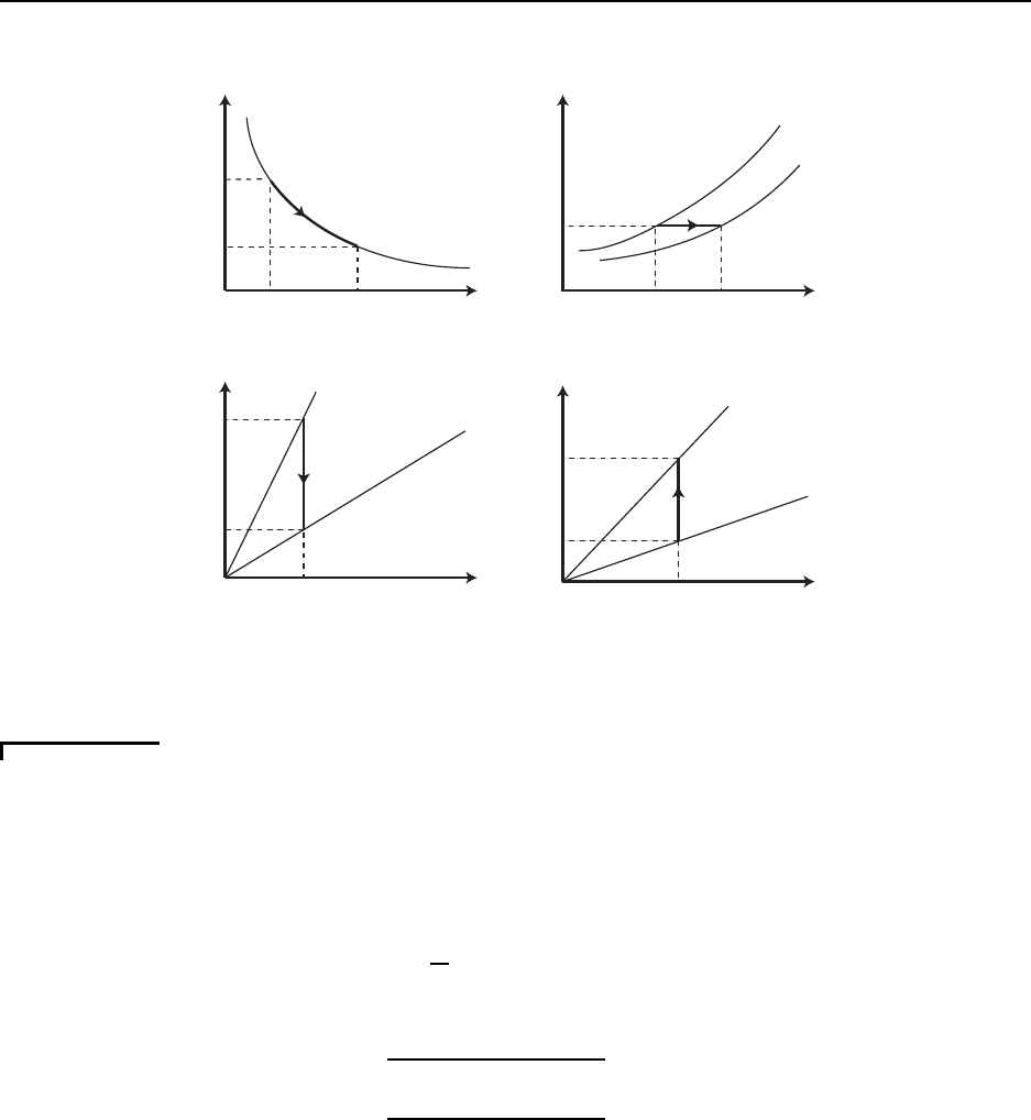
Figure 3.1 gives a sketch of an isothermal thermodynamic process going from state 1 to
state 2. The figure shows a variety of planes, P − v, T − s, P − T , and v − T . For ideal
gases, 1) isotherms are hyperbola s in the P −v plane: P = (RT ) /v, 2) isochores are straight
lines in the P − T plane: P = (R/v)T , with large v giving a small slope, and 3 ) isobars
are straight lines in the v − T plane: v = (RT )/P , with large P g iving a small slope. The
area under the curve in the P − v plane gives the work. The area under t he curve in the
T −s plane gives the heat tra nsfer. The energy change is given by the difference in the heat
transfer and the work. The isochores in the T − s plane are non-trivial. For a calorically
perfect ideal g as, they are given by exponential curves.
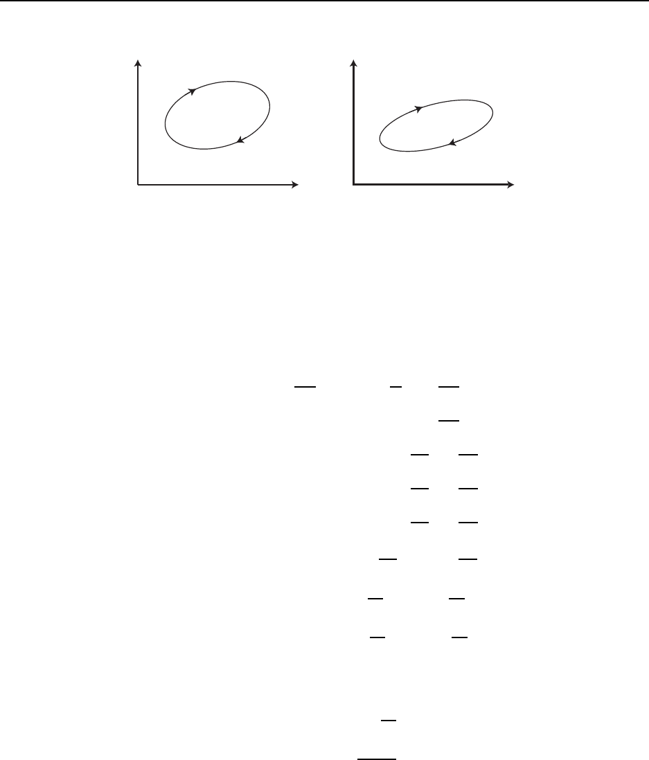
Figure 3.2 gives a sketch of a t hermodynamic cycle. Here we only sketch the P − v and
T − s planes, though others could be included. Since it is a cyclic process, there is no net
energy change for the cycle and the cyclic work equals the cyclic heat transfer. The enclosed
area in the P − v plane, i.e. the net work, equals the enclosed ar ea in the T − s plane, i.e.
the net heat transfer. The sketch has the cycle working in the direction which corresponds
to an engine. A reversal of the direction would correspond to a refrigerator.
CC BY-NC-ND. 28 October 2019, J. M. Powers.
3.2. SUMMARY OF THERMODYNAMIC CONCEPTS 41
v
P
T = T
1
v
2
v
1
12
12
2
1
∫
w = P dv
12
1
2
s
T
∫
q = T ds
12
1
2
e - e = q - w
v
2
v
1
s
2
s
1
T
P
T
v
v
1
v
2
2
T = T
1
v
1
v
2
2
1
2
P
P
1
P
2
P
T = T
1 2
2
T = T
1
1
P
2
P
Figure 3.1: Sketch of isothermal thermodynamic process
Example 3. 1
Consider the following isobaric process for air, modelled as a calorically perfect ideal gas, from state
1 to state 2. P
1
= 100 kP a, T
1
= 300 K, T
2
= 400 K.
Since the process is isobaric P = 100 kP a describes a s traight line in P −v and P − T planes and
P
2
= P
1
= 100 kP a. Since idea l gas, v − T plane:
v =
R
P
T straight lines! (3.7)
v
1
= RT
1
/P
1
=
(287 J/kg/K) (300 K)
100, 000 P a
= 0.861 m
3
/kg (3.8)
v
2
= RT
2
/P
2
=
(287 J/kg/K) (400 K)
100, 000 P a
= 1.148 m
3
/kg (3.9)
Since calorically perfect:
de = c
v
dT (3.10)
Z
e
1
e
2
de = c
v
Z
T
1
T
2
dT (3.11)
e
2
− e
1
= c
v
(T
2
− T
1
) (3.12)
= (716.5 J/kg/K) (400 K − 300 K) (3.13)
= 71, 650 J/kg (3.14)
CC BY-NC-ND. 28 October 2019, J. M. Powers.
42 CHAPTER 3. THERMODYNAMICS REVIEW
v
P
s
T
q = w
cycle
cycle
Figure 3.2: Sketch of thermodynamic cycle
also
T ds = de + P dv (3.15)
T ds = c
v
dT + P dv (3.16)
from ideal gas : v =
RT
P
: dv =
R
P
dT −
RT
P
2
dP (3.17)
T ds = c
v
dT + RdT −
RT
P
dP (3.18)
ds = (c
v
+ R)
dT
T
− R
dP
P
(3.19)
ds = (c
v
+ c
p
− c
v
)
dT
T
− R
dP
P
(3.20)
ds = c
p
dT
T
− R
dP
P
(3.21)
Z
s
2
s
1
ds = c
p
Z
T
2
T
1
dT
T
− R
Z
P
2
P
1
dP
P
(3.22)
s
2
− s
1
= c
p
ln
T
2
T
1
− R ln
P
2
P
1
(3.23)
s − s
o
= c
p
ln
T
T
o
− R ln
P
P
o
(3.24)
since P = constant: (3.25)
s
2
− s
1
= c
p
ln
T
2
T
1
(3.26)
= (1003.5 J/kg/K) ln
400 K
300 K
(3.27)
= 288.7 J/kg/K (3.28)
w
12
=
Z
v
2
v
1
P dv = P
Z
v
2
v
1
dv (3.29)
= P (v
2
− v
1
) (3.30)
CC BY-NC-ND. 28 October 2019, J. M. Powers.

3.2. SUMMARY OF THERMODYNAMIC CONCEPTS 43
= (100, 0 00 P a)(1.148 m
3
/kg − 0.861 m
3
/kg) (3.31)
= 29, 600 J/kg (3.32)
Now
de = δq − δw (3.33)
δq = de + δw (3.34)
q
12
= (e
2
− e
1
) + w
12
(3.35)
q
12
= 71, 650 J/kg + 29, 600 J/kg (3.36)
q
12
= 101, 250 J/kg (3.37)
Now in this process the gas is heated from 300 K to 40 0 K. We would expect at a minimum that the
surroundings were at 400 K. Let’s check for second law satisfaction.
s
2
− s
1
≥
q
12
T
surr
? (3.38)
288.7 J/kg/K ≥
101, 250 J/kg
400 K
? (3.39)
288.7 J/kg/K ≥ 253.1 J/kg/K yes (3.40)
v
P
T = 300 K
1
T
2
v
2
v
1
P = P = 100 kPa
1
2
12
12
2
1
∫
w = P dv
12
1
2
s
T
∫
q = T ds
12
1
2
e - e = q - w
v
2
v
1
s
2
s
1
T
T
1
2
T
P
T
v
v
1
v
2
T
2
T
1
P = P = 100 kPa
1
2
P = P = 100 kPa
1
2
T
1
T
2
v
1
v
2
Figure 3.3: Sketch for isobaric example problem
CC BY-NC-ND. 28 October 2019, J. M. Powers.

44 CHAPTER 3. THERMODYNAMICS REVIEW
3.3 Maxwell relations and sec ondary properties
Recall
de = T ds − P d
1
ρ
(3.41)
Since v ≡ 1/ ρ we get
de = T ds −P d v (3.42)
Now we assume e = e(s, v),
de =
∂e
∂s
v
ds +
∂e
∂v
s
dv (3.43)
Thus
T =
∂e
∂s
v
P = −
∂e
∂v
s
(3.44)
and
∂T
∂v
s
=
∂
2
e
∂v∂s
∂P
∂s
v
= −
∂
2
e
∂s∂v
(3.45)
Thus we get a Maxwell relation:
∂T
∂v
s
= −
∂P
∂s
v
(3.46)
Define the following properties:
• enthalpy: h ≡ e + pv
• Helmholtz free energy: a ≡ e − T s
• Gibbs free energy: g ≡ h − T s
Now with these definitions it is easy to form differential relations using the Gibbs relation
as a root.
h = e + P v (3.47)
dh = de + P dv + vdP (3.48)
de = dh − P dv − vdP (3 .49)
substitute into Gibbs: de = T ds − P d v (3.50)
dh − P dv − vdP = T ds − P dv (3.51)
dh = T ds + vdP (3.52)
CC BY-NC-ND. 28 October 2019, J. M. Powers.

3.3. MAXWELL RELATIONS AND SECONDARY PROPERTIES 45
So s and P are nat ural var iables for h. Through a very similar process we get the following
relationships:
∂h
∂s
P
= T
∂h
∂P
s
= v (3.53)
∂a
∂v
T
= −P
∂a
∂T
v
= −s (3.54)
∂g
∂P
T
= v
∂g
∂T
P
= −s (3.55)
∂T
∂P
s
=
∂v
∂s
P
∂P
∂T
v
=
∂s
∂v
T
∂v
∂T
P
= −
∂s
∂P
T
(3.56)
The following thermodynamic properties are also useful and have formal definitions:
• specific heat at constant volume: c
v
≡
∂e
∂T
v
• specific heat at constant pressure: c
p
≡
∂h
∂T
P
• ratio of specific heats: γ ≡ c
p
/c
v
• sound speed: c ≡
r
∂P
∂ρ
s
• adiabatic compressibility: β
s
≡ −
1
v
∂v
∂P
s
• adiabatic bulk modulus: B
s
≡ −v
∂P
∂v
s
Generic problem: given P = P (T, v), find other properties
3.3.1 Internal energy from thermal equation of state
Find the internal energy e(T, v) for a general material.
e = e(T, v) (3.57)
de =
∂e
∂T
v
dT +
∂e
∂v
T
dv (3.58)
de = c
v
dT +
∂e
∂v
T
dv (3.59)
Now from Gibbs,
de = T ds −P d v (3.6 0)
de
dv
= T
ds
dv
− P (3.61)
∂e
∂v
T
= T
∂s
∂v
T
− P (3.62)
CC BY-NC-ND. 28 October 2019, J. M. Powers.

46 CHAPTER 3. THERMODYNAMICS REVIEW
Substitute from Maxwell relation,
∂e
∂v
T
= T
∂P
∂T
v
− P (3.63)
so
de = c
v
dT +
T
∂P
∂T
v
− P
dv (3.64)
Z
e
e
o
dˆe =
Z
T
T
o
c
v
(
ˆ
T )d
ˆ
T +
Z
v
v
o
ˆ
T
∂
ˆ
P
∂
ˆ
T
ˆv
−
ˆ
P
!
dˆv (3.65)
e(T, v) = e
o
+
Z
T
T
o
c
v
(
ˆ
T )d
ˆ
T +
Z
v
v
o
ˆ
T
∂
ˆ
P
∂
ˆ
T
ˆv
−
ˆ
P
!
dˆv (3.66)
Example 3. 2
Ideal gas
Find a general expre ssion for e(T, v) if
P (T, v) =
RT
v
(3.67)
Proceed as follows:
∂P
∂T
v
= R/v (3.68)
T
∂P
∂T
v
− P =
RT
v
− P (3.69)
=
RT
v
−
RT
v
= 0 (3.70)
Thus e is
e(T ) = e
o
+
Z
T
T
o
c
v
(
ˆ
T )d
ˆ
T (3.71)
We also find
h = e + P v = e
o
+
Z
T
T
o
c
v
(
ˆ
T )d
ˆ
T + Pv (3.72)
h(T, v) = e
o
+
Z
T
T
o
c
v
(
ˆ
T )d
ˆ
T + RT (3.73)
c
p
(T, v) =≡
∂h
∂T
P
= c
v
(T ) + R = c
p
(T ) (3.74)
R = c
p
(T ) − c
v
(T ) (3.75)
Iff c
v
is a constant then
e(T ) = e
o
+ c
v
(T − T
o
) (3.76)
h(T ) = (e
o
+ P
o
v
o
) + c
p
(T − T
o
) (3.77)
R = c
p
− c
v
(3.78)
CC BY-NC-ND. 28 October 2019, J. M. Powers.

3.3. MAXWELL RELATIONS AND SECONDARY PROPERTIES 47
Example 3. 3
van der Waals gas
Find a general expre ssion for e(T, v) if
P (T, v) =
RT
v − b
−
a
v
2
(3.79)
Proceed as before :
∂P
∂T
v
=
R
v − b
(3.80)
T
∂P
∂T
v
− P =
RT
v − b
− P (3.81)
=
RT
v − b
−
RT
v − b
−
a
v
2
=
a
v
2
(3.82)
Thus e is
e(T, v) = e
o
+
Z
T
T
o
c
v
(
ˆ
T )d
ˆ
T +
Z
v
v
o
a
ˆv
2
dˆv (3.83)
= e
o
+
Z
T
T
o
c
v
(
ˆ
T )d
ˆ
T + a
1
v
o
−
1
v
(3.84)
We also find
h = e + P v = e
o
+
Z
T
T
o
c
v
(
ˆ
T )d
ˆ
T + a
1
v
o
−
1
v
+ Pv (3.85 )
h(T, v) = e
o
+
Z
T
T
o
c
v
(
ˆ
T )d
ˆ
T + a
1
v
o
−
1
v
+
RT v
v − b
−
a
v
(3.86)
(3.87)
3.3.2 Sound speed from thermal equation of state
Find the sound speed c(T, v) f or a general material.
c =
s
∂P
∂ρ
s
(3.88)
c
2
=
∂P
∂ρ
s
(3.89)
CC BY-NC-ND. 28 October 2019, J. M. Powers.

48 CHAPTER 3. THERMODYNAMICS REVIEW
Use Gibbs relation
T ds = de + P dv (3.90)
(3.91)
Substitute earlier r elat ion for de
T ds =
c
v
dT +
T
∂P
∂T
v
− P
dv
+ P dv (3.92)
T ds = c
v
dT + T
∂P
∂T
v
dv (3.93)
T ds = c
v
dT −
T
ρ
2
∂P
∂T
ρ
dρ (3.94)
Since P = P (T, v), P = P (T, ρ)
dP =
∂P
∂T
ρ
dT +
∂P
∂ρ
T
dρ (3.95)
dT =
dP −
∂P
∂ρ
T
dρ
∂P
∂T
ρ
(3.96)
Thus substituting for dT
T ds = c
v
dP −
∂P
∂ρ
T
dρ
∂P
∂T
ρ
−
T
ρ
2
∂P
∂T
ρ
dρ (3.97)
so g r ouping terms in dP and dρ we get
T ds =
c
v
∂P
∂T
ρ
!
dP −
c
v
∂P
∂ρ
T
∂P
∂T
ρ
+
T
ρ
2
∂P
∂T
ρ
dρ (3.98)
SO if ds ≡ 0 we obtain
∂P
∂ρ
s
=
1
c
v
∂P
∂T
ρ
c
v
∂P
∂ρ
T
∂P
∂T
ρ
+
T
ρ
2
∂P
∂T
ρ
(3.99)
=
∂P
∂ρ
T
+
T
c
v
ρ
2
∂P
∂T
ρ
!
2
(3.100)
So
c(T, ρ) =
v
u
u
t
∂P
∂ρ
T
+
T
c
v
ρ
2
∂P
∂T
ρ
!
2
(3.101)
CC BY-NC-ND. 28 October 2019, J. M. Powers.

3.3. MAXWELL RELATIONS AND SECONDARY PROPERTIES 49
Exercises: Liepmann and Roshko, 1.3 and 1.4, p. 383.
Example 3. 4
Ideal gas
Find the sound spe ed if
P (T, ρ) = ρRT (3.102)
The necessary partials are
∂P
∂ρ
T
= RT
∂P
∂T
ρ
= ρR (3.103)
so
c(T, ρ) =
s
RT +
T
c
v
ρ
2
(ρR)
2
(3.104)
=
s
RT +
R
2
T
c
v
(3.105)
=
s
RT
1 +
R
c
v
(3.106)
=
s
RT
1 +
c
P
− c
v
c
v
(3.107)
=
s
RT
c
v
+ c
P
− c
v
c
v
(3.108)
=
p
γRT (3.109)
Sound speed depends on temperature alone for the calorically p e rfect ideal gas.
Example 3. 5
Virial gas
Find the sound spe ed if
P (T, ρ) = ρRT (1 + b
1
ρ) (3.110)
The necessary partials are
∂P
∂ρ
T
= RT + 2b
1
ρRT
∂P
∂T
ρ
= ρR (1 + b
1
ρ) (3.111)
CC BY-NC-ND. 28 October 2019, J. M. Powers.

50 CHAPTER 3. THERMODYNAMICS REVIEW
so
c(T, ρ) =
s
RT + 2b
1
ρRT +
T
c
v
ρ
2
(ρR (1 + b
1
ρ))
2
(3.112)
=
s
RT
1 + 2b
1
ρ +
R
c
v
(1 + b
1
ρ)
2
(3.113)
Sound speed depends on both temperature and density.
Example 3. 6
Thermodynamic process with a van de r Waals Gas
A van der Waals ga s with
R = 200 J/ kg/K (3.114)
a = 150 P a m
6
/kg
2
(3.115)
b = 0.001 m
3
/kg (3.116)
c
v
= [350 + 0.2(T − 300K)] J/kg/K (3.117)
begins at T
1
= 300 K, P
1
= 1×10
5
P a . It is isothermally compressed to state 2 where P
2
= 1×10
6
P a .
It is then isochorically heated to state 3 where T
3
= 1, 000 K. Find w
13
, q
13
, and s
3
−s
1
. Assume the
surroundings are at 1, 000 K. Recall
P =
RT
v − b
−
a
v
2
(3.118)
so at state 1
100, 000 =
200 ×300
v
1
− 0.001
−
150
v
2
1
(3.119)
or expanding
−0.15 + 150v − 60, 100v
2
+ 100, 000v
3
= 0 (3.120)
Cubic equation–three solutions:
v
1
= 0.598 m
3
/kg (3.121)
v
1
= 0.00125 −0.0097i m
3
/kg not physical (3.122)
v
1
= 0.00125 + 0.0097i m
3
/kg not physical (3.123)
Now at state 2 we know P
2
and T
2
so we can deter mine v
2
1, 000, 000 =
200 ×300
v
2
− 0.001
−
150
v
2
2
(3.124)
The physical solution is v
2
= 0.0585 m
3
/kg. Now at state 3 we know v
3
= v
2
and T
3
. Determine P
3
:
P
3
=
200 ×1, 000
0.0585 −0.001
−
150
0.0585
2
= 3, 478, 261 − 43, 831 = 3 , 434, 430 P a (3.125)
CC BY-NC-ND. 28 October 2019, J. M. Powers.

3.3. MAXWELL RELATIONS AND SECONDARY PROPERTIES 51
Now w
13
= w
12
+ w
23
=
R
2
1
P dv +
R
3
2
P dv =
R
2
1
P dv since 2 − 3 is at constant volume. So
w
13
=
Z
v
2
v
1
RT
v − b
−
a
v
2
dv (3.126)
= RT
1
Z
v
2
v
1
dv
v − b
− a
Z
v
2
v
1
dv
v
2
(3.127)
= RT
1
ln
v
2
− b
v
1
− b
+ a
1
v
2
−
1
v
1
(3.128)
= 200 ×300 ln
0.0585 − 0.001
0.598 −0.001
+ 150
1
0.0585
−
1
0.598
(3.129)
= −140, 40 8 + 2, 313 (3.130)
= −138, 095 J/kg = −138 kJ/kg (3.131)
The gas is co mpressed, so the work is negative. Since e is a state prop erty:
e
3
− e
1
=
Z
T
3
T
1
c
v
(T )dT + a
1
v
1
−
1
v
3
(3.132)
Now
c
v
= 350 + 0.2(T − 300) = 290 +
1
5
T (3.133)
so
e
3
− e
1
=
Z
T
3
T
1
290 +
1
5
T
dT + a
1
v
1
−
1
v
3
(3.134)
= 290 (T
3
− T
1
) +
1
10
T
2
3
− T
2
1
+ a
1
v
1
−
1
v
3
(3.135)
290 (1, 000 −300) +
1
10
1, 000
2
− 300
2
+ 150
1
0.598
−
1
0.0585
(3.136)
= 203, 000 + 91, 000 − 2, 313 (3.137)
= 291, 687 J/kg = 292 kJ/kg (3.138)
Now from the first law
e
3
− e
1
= q
13
− w
13
(3.139)
q
13
= e
3
− e
1
+ w
13
(3.140)
q
13
= 292 −138 (3.141)
q
13
= 154 kJ/kg (3.142)
The heat transfer is positive as heat was added to the system.
Now find the entropy change. Manipulate the Gibbs equa tion:
T ds = de + P dv (3.143)
ds =
1
T
de +
P
T
dv (3.144)
ds =
1
T
c
v
(T )dT +
a
v
2
dv
+
P
T
dv (3.145)
CC BY-NC-ND. 28 October 2019, J. M. Powers.

52 CHAPTER 3. THERMODYNAMICS REVIEW
ds =
1
T
c
v
(T )dT +
a
v
2
dv
+
1
T
RT
v − b
−
a
v
2
dv (3.146)
ds =
c
v
(T )
T
dT +
R
v − b
dv (3.147)
s
3
− s
1
=
Z
T
3
T
1
c
v
(T )
T
dT + R ln
v
3
− b
v
1
− b
(3.148)
=
Z
1,000
300
290
T
+
1
5
dT + R ln
v
3
− b
v
1
− b
(3.149)
= 290 ln
1, 000
300
+
1
5
(1, 00 0 −300) + 200 ln
0.0585 −0.001
0.598 −0.001
(3.150)
= 349 + 140 −468 (3.151)
= 21
J
kg K
= 0.021
kJ
kg K
(3.152)
Is the second law satisfied for each portion of the process?
First look at 1 → 2
e
2
− e
1
= q
12
− w
12
(3.153)
q
12
= e
2
− e
1
+ w
12
(3.154)
q
12
=
Z
T
2
T
1
c
v
(T )dT + a
1
v
1
−
1
v
2
!
+
RT
1
ln
v
2
− b
v
1
− b
+ a
1
v
2
−
1
v
1
(3.155)
(3.156)
Since T
1
= T
2
and canc eling the terms in a we get
q
12
= RT
1
ln
v
2
− b
v
1
− b
= 200 ×300 ln
0.0585 −0.001
0.598 −0.001
= −140, 408
J
kg
(3.157)
Since isothermal
s
2
− s
1
= R ln
v
2
− b
v
1
− b
(3.158)
= 200 ln
0.0585 −0.001
0.598 −0.001
(3.159)
= −468.0
J
kg K
(3.160)
Entropy drops because heat was trans ferred out of the system.
Check the second law. Note that in this portion of the process in which the heat is transferred out
of the system, that the surroundings must have T
surr
≤ 300 K. For this portion of the process let us
take T
surr
= 300 K.
s
2
− s
1
≥
q
12
T
? (3.161)
−468.0
J
kg K
≥
−140, 408
J
kg
300 K
(3.162)
−468.0
J
kg K
≥ −468.0
J
kg K
ok (3.163)
CC BY-NC-ND. 28 October 2019, J. M. Powers.

3.4. CANONICAL EQUATIONS OF STATE 53
Next look at 2 → 3
q
23
= e
3
− e
2
+ w
23
(3.164)
q
23
=
Z
T
3
T
2
c
v
(T )dT + a
1
v
2
−
1
v
3
!
+
Z
v
3
v
2
P dv
(3.165)
since isochoric q
23
=
Z
T
3
T
2
c
v
(T )dT (3.166)
=
Z
1000
300
290 +
T
5
dT = 294, 000
J
K
(3.167)
Now look at the entropy change for the isochoric process:
s
3
− s
2
=
Z
T
3
T
2
c
v
(T )
T
dT (3.168)
=
Z
T
3
T
2
290
T
+
1
5
dT (3.169)
= 290 ln
1, 000
300
+
1
5
(1, 00 0 − 300) = 489
J
kg K
(3.170)
Entropy rises because heat transferred into system.
In order to transfer heat into the sy stem we must have a differ ent thermal reservoir. This one must
have T
surr
≥ 1000 K. Assume here that the heat transfer was fr om a reservoir held at 1, 000 K to
assess the influence o f the second law.
s
3
− s
2
≥
q
23
T
? (3.171)
489
J
kg K
≥
294, 000
J
kg
1, 000 K
(3.172)
489
J
kg K
≥ 294
J
kg K
ok (3.173)
3.4 Canonical equations of state
If we have a single equation of state in a special canonical form, we can form both thermal
and caloric equations. Since
de = T ds − P d v (3.17 4)
dh = T ds + vdP (3.175)
it is suggested that the form
e = e(s, v ) (3.176)
h = h( s , P ) (3.177)
CC BY-NC-ND. 28 October 2019, J. M. Powers.

54 CHAPTER 3. THERMODYNAMICS REVIEW
is useful.
Example 3. 7
Canonical Form
If
h(s, P ) = Kc
p
P
R/c
p
exp
s
c
p
+ (h
o
− c
p
T
o
) (3.178)
derive both thermal and caloric sta te equations P (v, T ) and e(v, T ).
Now for our material
∂h
∂s
P
= KP
R/c
p
exp
s
c
p
(3.179)
∂h
∂P
s
= KRP
R/c
p
−1
exp
s
c
p
(3.180)
Now since
∂h
∂s
P
= T (3.181)
∂h
∂P
s
= v (3.182)
we have
T = KP
R/c
p
exp
s
c
p
(3.183)
v = KRP
R/c
p
−1
exp
s
c
p
(3.184)
Dividing one by the other gives
T
v
=
P
R
(3.185)
P =
RT
v
(3.186)
Substituting our expression for T into our canonical equation for h we also get
h = c
p
T + (h
o
− c
p
T
o
) (3.187)
h = c
p
(T − T
o
) + h
o
(3.188)
which is useful in itself. Substituting in for T and T
o
h = c
p
P v
R
−
P
o
v
o
R
+ h
o
(3.189)
Using h ≡ e + P v we get
e + P v = c
p
P v
R
−
P
o
v
o
R
+ e
o
+ P
o
v
o
(3.190)
CC BY-NC-ND. 28 October 2019, J. M. Powers.

3.5. ISENTROPIC RELATIONS 55
so
e =
c
p
R
− 1
P v −
c
p
R
− 1
P
o
v
o
+ e
o
(3.191)
e =
c
p
R
− 1
(P v − P
o
v
o
) + e
o
(3.192)
e =
c
p
R
− 1
(RT − RT
o
) + e
o
(3.193)
e = (c
p
− R) (T − T
o
) + e
o
(3.194)
e = [c
p
− (c
p
− c
v
)] (T − T
o
) + e
o
(3.195)
e = c
v
(T − T
o
) + e
o
(3.196)
So one canonical equa tion gives us all the information we nee d! Oftentimes, it is difficult to do a
single experiment to g et the canonical form.
Exercise: For a calorically perfect ideal gas, write the Helmholtz free energy and Gibbs
free energy in canonical form, i.e. what is a(T, v), g(P, T )?
3.5 Isentropic relations
Of particular importance in thermodynamics in general and compressible flow in particular
are relations that describe an isentropic process, s = constant. Recall the second law.
ds ≥
δq
T
(3.197)
If the process is reversible,
ds =
δq
T
(3.198)
If the process is adiabatic
δq ≡ 0 so ds = 0 (3.199)
So an isentropic process is both adiabatic and reversible. We know from the first law written
in terms of entropy that this implies that
q ≡ 0 (3.200)
τ ≡ 0 (3.201)
In this case the Gibbs relation and the first law reduce to the same expression:
de = −P dv (3.202)
That is the energy change is all due to reversible pressure volume work.
We would like to develop an expression between two variables for a n isentropic process.
With knowledge of P (T, v)
CC BY-NC-ND. 28 October 2019, J. M. Powers.

56 CHAPTER 3. THERMODYNAMICS REVIEW
• form e(T, v)
• eliminate T to form e(P, v)
• take derivative and substitute into Gibbs/First Law
∂e
∂P
v
dP +
∂e
∂v
P
dv = −P dv (3.203)
∂e
∂P
v
dP +
∂e
∂v
P
+ P
dv = 0 (3.204)
Integration of this equation gives a relatio nship between P and v.
Example 3. 8
Calorically Perfect Ideal Gas
Find the relationship fo r a calorically perfect ideal gas which undergoes an isentropic process.
Ideal Gas:
P v = RT (3.205)
Calorically Perfect:
e = c
v
T + e
o
(3.206)
Thus
e = c
v
P v
R
+ e
o
=
c
v
c
P
− c
v
P v + e
o
=
1
γ − 1
P v + e
o
(3.207)
Thus the necessary derivatives are
∂e
∂P
v
=
1
γ − 1
v (3.208)
∂e
∂v
P
=
1
γ − 1
P (3.209)
so s ubstituting into our developed relatio nship gives
1
γ − 1
vdP +
1
γ − 1
P + P
dv = 0 (3.210)
vdP + γP dv = 0 (3.211)
dP
P
= −γ
dv
v
(3.212)
ln
P
P
o
= −γ ln
v
v
o
(3.213)
ln
P
P
o
= ln
v
o
v
γ
(3.214)
P
P
o
=
v
o
v
γ
(3.215)
P v
γ
= P
o
v
γ
o
= constant (3.216)
CC BY-NC-ND. 28 October 2019, J. M. Powers.

3.5. ISENTROPIC RELATIONS 57
also using the thermal state equation
P
P
o
=
RT
v
RT
o
v
o
=
T
T
o
v
o
v
=
v
o
v
γ
(3.217)
T
T
o
=
v
o
v
γ− 1
=
P
P
o
γ−1
γ
(3.218)
Find the work in a process from v
1
to v
2
w
12
=
Z
1
2
P dv (3.219)
= P
o
v
γ
o
Z
v
2
v
1
dv
v
γ
(3.220)
= P
o
v
γ
o
v
1−γ
1 −γ
v
2
v
1
(3.221)
=
P
o
v
γ
o
1 −γ
v
1−γ
2
− v
1−γ
1
(3.222)
=
P
2
v
2
− P
1
v
1
1 −γ
(3.223)
Also
de = δq − δw = 0 − δw so (3.224)
e
2
− e
1
=
P
2
v
2
− P
1
v
1
γ − 1
(3.225)
Figure 3.4 gives a sketch for the calorically perfect ideal gas undergoing an isentropic
expansion in various pla nes.
Example 3. 9
Virial Gas
Find the relationship between P and v for a virial gas with constant c
v
which undergoes an isentropic
process.
Virial Gas:
P =
RT
v − b
(3.226)
This is van der Waals with a = 0 and c
v
constant so:
e = c
v
T + e
o
(3.227)
Thus
e = c
v
P (v − b)
R
+ e
o
(3.228)
CC BY-NC-ND. 28 October 2019, J. M. Powers.

58 CHAPTER 3. THERMODYNAMICS REVIEW
v
P
T
2
T
1
v
2
v
1
12
12
2
1
∫
w = P dv
12
1
2
s
T
∫
q = T ds
12
1
2
e - e = q - w
v
2
v
1
s
2
s =
1
T
T
1
2
T
P
T
v
v
1
v
2
T
1
T
2
T
1
T
2
v
1
v
2
P
P
1
2
P
2
P
1
P
P
1
2
Figure 3.4: Sketch of isent ropic expansion process
Thus the necessary derivatives are
∂e
∂P
v
=
c
v
R
(v − b) (3.229)
∂e
∂v
P
=
c
v
R
P (3.230)
so s ubstituting into our developed relatio nship gives
c
v
R
(v − b) dP +
c
v
R
P + P
dv = 0 (3.231)
(v − b) dP +
1 +
R
c
v
P dv = 0 (3.232)
with ˆγ ≡ 1 +
R
c
v
(3.233)
dP
dv
+
ˆγ
v − b
P = 0 (3.234)
exp
Z
ˆγ
v − b
dv
dP
dv
+
exp
Z
ˆγ
v − b
dv
ˆγ
v − b
P = 0 (3.235)
exp
ln (v − b)
ˆγ
dP
dv
+
exp
ln (v − b)
ˆγ
ˆγ
v − b
P = 0 (3.236)
(v − b)
ˆγ
dP
dv
+ (v − b)
ˆγ
ˆγ
v − b
P = 0 (3.237)
d
dv
(v − b)
ˆγ
P
= 0 (3.238)
CC BY-NC-ND. 28 October 2019, J. M. Powers.

3.5. ISENTROPIC RELATIONS 59
(v − b)
ˆγ
P = (v
o
− b)
ˆγ
P
o
(3.239)
P
P
o
=
v
o
− b
v − b
ˆγ
(3.240)
Exercise: Find the relationship between T and v for a virial gas in an isentropic process.
Exercise: Find an expression for the work done by a van der Waals gas in an isentropic
process.
Exercise: A virial gas, m = 3 kg with R = 290
J
kgK
, b = 0.002
m
3
kg
with constant specific
heat c
v
= 0.700
kJ
kg K
is initially at P = 1.2 bar a nd T = 320 K. It undergoes a two step
process: 1 → 2 is an isochoric compression to 500 kP a; 2 → 3 is a n isentropic expansion to
300 kP a. F ind the total work W
13
in units of J, the total heat transfer Q
13
in units of J,
and the change in ent r opy S
3
−S
1
in units of J/K. Include a sketch, roughly to scale, of the
total process in the P − v a nd T − s planes.
CC BY-NC-ND. 28 October 2019, J. M. Powers.

Chapter 4
One-dimensional compressible flow
White, Chapter 9: pp. 511-559,
Liepmann and Roshko, Chapter 2: pp. 39-65,
Hughes and Brighton, Chapter 7: pp. 178-185,
Shapiro, Vol. 1, Chapters 4-8: pp. 73-262,
This chapter will discuss one-dimensional flow of a compressible fluid. Notation can pose
problems, and many common ones are in use. Here a new convention will be adopted. In
this chapter
• velocity in the x-direction will be denoted as u,
• specific internal energy, denoted in previous chapters by u, will here be e,
• total internal energy, denoted in previous chapters by U, will here be E.
The following topics will be covered:
• development of g eneralized one- dimensional flow equations,
• isentropic flow with area change,
• flow with nor ma l shock waves,
• flow with fr ictio n (Fanno flow),
• flow with heat transfer (Rayleigh flow),
• flow in a shock tube.
Assume for this chapter:
• The flow is uni-dir ectional in the x− direction with u 6= 0 and with the y− and z−
components of the velocity vector both zero: v ≡ 0 , w ≡ 0
61

62 CHAPTER 4. ONE-DIMENSIONAL COMPRESSIBLE FLOW
• Spatial g r adients are admitted in x, but not in y or z:
∂
∂x
6= 0,
∂
∂y
≡ 0,
∂
∂z
≡ 0.
Friction and heat transfer will not be modelled r igorously. Instead, they will be modelled
in a fashion which captures the relevant physics and retains analytic tra cta bility.
4.1 Generalized one-dimensio nal equations
Flow with area change is illustrated by the following sketch of a control volume:. See Figure
4.1.
ρ
u
A
P
e
1
1
1
1
1
ρ
u
A
P
e
2
2
2
2
2
x
1
x
2
x - x = ∆ x
2
1
q
τ
w
Perimeter = L
Figure 4.1: Control volume sketch
For this problem a dopt the following conventions
• surface 1 a nd 2 are o pen and allow fluxes of mass, momentum, and energy
• surface w is a closed wall; no mass flux through the wall
• external heat flux q
w
(Energy/Area/Time:
W
m
2
) through the wall allowed-q
w
known fixed
parameter
• diffusive, longitudinal heat transfer ignored, q
x
= 0
• wall shear τ
w
(Force/Area:
N
m
2
) allowed–τ
w
known, fixed parameter
• diffusive viscous stress not allowed τ
xx
= 0
• cross-sectional area a known fixed function: A(x)
CC BY-NC-ND. 28 October 2019, J. M. Powers.

4.1. GENERALIZED ONE-DIMENSIONAL EQUATIONS 63
4.1.1 Mass
Take the overbar notation to indicate a volume averaged quantity.
The amount of mass in a control volume after a time increment ∆t is equal to the original
amount of mass plus that which came in minus that which left:
¯ρ
¯
A∆x
t+∆t
= ¯ρ
¯
A∆x
t
+ ρ
1
A
1
(u
1
∆t) − ρ
2
A
2
(u
2
∆t) (4.1)
Rearrange and divide by ∆x∆t:
¯ρ
¯
A
t+∆t
− ¯ρ
¯
A
t
∆t
+
ρ
2
A
2
u
2
− ρ
1
A
1
u
1
∆x
= 0 (4.2)
(4.3)
Taking the limit as ∆t → 0, ∆x → 0:
∂
∂t
(ρA) +
∂
∂x
(ρAu) = 0 (4.4)
If steady
d
dx
(ρAu) = 0 (4.5)
Au
dρ
dx
+ ρu
dA
dx
+ ρA
du
dx
= 0 (4.6)
1
ρ
dρ
dx
+
1
A
dA
dx
+
1
u
du
dx
= 0 (4.7)
Integrate from x
1
to x
2
:
Z
x
2
x
1
d
dx
(ρAu)dx =
Z
x
2
x
1
0dx (4.8)
Z
2
1
d (ρAu) = 0 (4.9)
ρ
2
u
2
A
2
− ρ
1
u
1
A
1
= 0 (4.10)
ρ
2
u
2
A
2
= ρ
1
u
1
A
1
≡ ˙m = C
1
(4.11)
4.1.2 Momentum
Newton’s Second L aw says the time rate of change of linear momentum of a body equals the
sum of the forces acting on the body. In the x direction this is roughly as follows:
d
dt
(mu) = F
x
(4.12)
CC BY-NC-ND. 28 October 2019, J. M. Powers.

64 CHAPTER 4. ONE-DIMENSIONAL COMPRESSIBLE FLOW
In discrete form this would be
mu|
t+∆t
− mu|
t
∆t
= F
x
(4.13)
mu|
t+∆t
= mu|
t
+ F
x
∆t (4.14)
For a control volume containing fluid, one must also account for the momentum which
enters and leaves the control volume. The amount of momentum in a control volume after
a time increment ∆t is equal to the original amount of momentum plus that which came in
minus that which left plus that introduced by the fo r ces acting on the control volume.
• pressure force at surface 1 pushes fluid
• pressure force at surface 2 restrai ns fluid
• force due to the reaction of the wall to the pressure force pushes fluid if area change
positive
• force due to the reaction of the wall to the shear force restrai ns fluid
¯ρ
¯
A∆x
¯u
t+∆t
=
¯ρ
¯
A∆x
¯u
t
+ (ρ
1
A
1
(u
1
∆t)) u
1
−(ρ
2
A
2
(u
2
∆t)) u
2
+ (P
1
A
1
) ∆t − (P
2
A
2
) ∆t
+
¯
P ( A
2
− A
1
)
∆t
−
τ
w
¯
L∆x
∆t
Rearrange and divide by ∆x∆t:
¯ρ
¯
A¯u
t+∆t
− ¯ρ
¯
A¯u
t
∆t
+
ρ
2
A
2
u
2
2
− ρ
1
A
1
u
2
1
∆x
= −
P
2
A
2
− P
1
A
1
∆x
+
¯
P
A
2
− A
1
∆x
− τ
w
¯
L
In the limit ∆x → 0, ∆t → 0 one gets
∂
∂t
(ρAu) +
∂
∂x
ρAu
2
= −
∂
∂x
(P A) + P
∂A
∂x
− τ
w
L (4.15)
In steady state:
d
dx
ρAu
2
= −
d
dx
(P A) + P
dA
dx
− τ
w
L (4.16)
CC BY-NC-ND. 28 October 2019, J. M. Powers.

4.1. GENERALIZED ONE-DIMENSIONAL EQUATIONS 65
ρAu
du
dx
+ u
d
dx
(ρAu) = −P
dA
dx
− A
dP
dx
+ P
dA
dx
− τ
w
L (4.17)
ρu
du
dx
= −
dP
dx
− τ
w
L
A
(4.18)
ρudu + dP = −τ
w
L
A
dx (4.19)
du +
1
ρu
dP = −τ
w
L
˙m
dx (4.20)
ρd
u
2
2
+ dP = −τ
w
L
A
dx (4.21)
Wall shear lowers the combination of pressure a nd dynamic head.
If no wall shear:
dP = −ρd
u
2
2
(4.22)
Increase in velocity magnitude decreases the pressure.
If no area change dA = 0 and no friction τ
w
≡ 0:
ρu
du
dx
+
dP
dx
= 0 (4.23)
add u mass u
d
dx
(ρu) = 0 (4.24)
d
dx
ρu
2
+ P
= 0 (4.25)
ρu
2
+ P = ρ
o
u
2
o
+ P
o
= C
2
(4.26)
4.1.3 Energy
The first law of thermodynamics states that the change of total energy of a body equals the
heat t ransferred to the body minus the work done by the body:
E
2
− E
1
= Q − W (4.27)
E
2
= E
1
+ Q − W (4.28)
So for the control volume this becomes the following when one also accounts for the energy
flux in and out of the control volume in addition to the work and heat transfer:
¯ρ
¯
A∆x
¯e +
¯u
2
2
t+∆t
=
¯ρ
¯
A∆x
¯e +
¯u
2
2
t
+ρ
1
A
1
(u
1
∆t)
e
1
+
u
2
1
2
− ρ
2
A
2
(u
2
∆t)
e
2
+
u
2
2
2
+q
w
¯
L∆x
∆t + (P
1
A
1
) (u
1
∆t) − (P
2
A
2
) (u
2
∆t)
CC BY-NC-ND. 28 October 2019, J. M. Powers.

66 CHAPTER 4. ONE-DIMENSIONAL COMPRESSIBLE FLOW
Note:
• mean pressure times area difference does no work because acting on stat ionary bound-
ary
• work done by shear force not included
1
Rearrange and divide by ∆t∆x:
¯ρ
¯
A
¯e +
¯u
2
2
t+∆t
− ¯ρ
¯
A
¯e +
¯u
2
2
t
∆t
+
ρ
2
A
2
u
2
e
2
+
u
2
2
2
+
P
2
ρ
2
− ρ
1
A
1
u
1
e
1
+
u
2
1
2
+
P
1
ρ
1
∆x
= q
w
¯
L
In differential form as ∆x → 0, ∆t → 0
∂
∂t
ρA
e +
u
2
2
+
∂
∂x
ρAu
e +
u
2
2
+
P
ρ
= q
w
L
In steady state:
d
dx
ρAu
e +
u
2
2
+
P
ρ
= q
w
L (4.29)
ρAu
d
dx
e +
u
2
2
+
P
ρ
+
e +
u
2
2
+
P
ρ
d
dx
(ρAu) = q
w
L (4.30)
ρu
d
dx
e +
u
2
2
+
P
ρ
=
q
w
L
A
(4.31)
ρu
de
dx
+ u
du
dx
+
1
ρ
dP
dx
−
P
ρ
2
dρ
dx
=
q
w
L
A
(4.32)
subtract product o f momentum and velocity (4.33)
ρu
2
du
dx
+ u
dP
dx
= −
τ
w
Lu
A
(4.34)
ρu
de
dx
−
P u
ρ
dρ
dx
=
q
w
L
A
+
τ
w
Lu
A
(4.35)
de
dx
−
P
ρ
2
dρ
dx
=
(q
w
+ τ
w
u) L
˙m
(4.36)
1
In neglecting work done by the wall shear force, I have taken an approach which is nearly universal, but
fundamentally difficult to defend. At this stage of the development of these notes, I am not ready to enter
into a grand battle with all established authors and proba bly confuse the student; consequently, results fo r
flow with friction w ill be consistent with those of other sources. The argument typically us ed to justify this
is that the real fluid satisfies no-slip a t the boundary; thus, the wall shear actually does no work. However,
one can easily argue that within the context o f the one-dimensional model which has been posed that the
shear force behaves as an external force which reduces the fluid’s mechanical energy. Moreover, it is possible
to show that neglect of this term results in the loss of fr ame invariance, a serious defect indeed. To model
the work of the wall shear , one would include the term
τ
w
¯
L∆x
(¯u∆t) in the e ne rgy equation.
CC BY-NC-ND. 28 October 2019, J. M. Powers.

4.1. GENERALIZED ONE-DIMENSIONAL EQUATIONS 67
Since e = e(P, ρ)
de =
∂e
∂ρ
P
dρ +
∂e
∂P
ρ
dP ( 4.37)
de
dx
=
∂e
∂ρ
P
dρ
dx
+
∂e
∂P
ρ
dP
dx
(4.38)
so
∂e
∂ρ
P
dρ
dx
+
∂e
∂P
ρ
dP
dx
−
P
ρ
2
dρ
dx
=
(q
w
+ τ
w
u) L
˙m
(4.39)
dP
dx
+
∂e
∂ρ
P
−
P
ρ
2
∂e
∂P
ρ
dρ
dx
=
(q
w
+ τ
w
u) L
˙m
∂e
∂P
ρ
(4.40)
Now it can be shown tha t
c
2
=
∂P
∂ρ
s
= −
∂e
∂ρ
P
−
P
ρ
2
∂e
∂P
ρ
(4.41)
so
dP
dx
− c
2
dρ
dx
=
(q
w
+ τ
w
u) L
˙m
∂e
∂P
ρ
(4.42)
dP
dx
− c
2
dρ
dx
=
(q
w
+ τ
w
u) L
ρuA
∂e
∂P
ρ
(4.43)
Special case of flow with no heat transfer q
w
≡ 0. Area change allowed!, wall friction
allowed! ( see earlier foot note):
ρu
d
dx
e +
u
2
2
+
P
ρ
= 0 (4.44)
e +
u
2
2
+
P
ρ
= e
o
+
u
2
o
2
+
P
o
ρ
o
= C
3
(4.45)
h +
u
2
2
= h
o
+
u
2
o
2
= C
3
(4.46)
Example 4. 1
Adiabatic Flow of Argon
2
2
adopted from White’s 9.1, p. 583
CC BY-NC-ND. 28 October 2019, J. M. Powers.

68 CHAPTER 4. ONE-DIMENSIONAL COMPRESSIBLE FLOW
Given: Argon, γ =
5
3
, flows adiabatically through a duct. At section 1, P
1
= 200 psia, T
1
=
500
◦
F, u
1
= 250
ft
s
. At section 2 P
2
= 40 psia, u
2
= 1, 100
ft
s
.
Find: T
2
in
◦
F and s
2
− s
1
in
Btu
lbm
◦
R
Assume: Ar is a calorically perfect ideal gas, tables give R = 38.68
ft lbf
lbmR
, c
p
= 0.1253
Btu
lbmR
Analysis: First get the units into shape:
T
1
= 500 + 460 = 960 R (4.47)
c
p
=
0.1253
Btu
lbm R
779
ft lbf
Btu
32.17
lbm f t
lbf s
2
= 3, 140
ft
2
s
2
R
(4.48)
R =
38.68
ft lbf
lbm R
32.17
lbm f t
lbf s
2
= 1, 244
ft
2
s
2
R
(4.49)
R =
38.68
ft lbf
lbm R
1
779
Btu
ft lbf
= 0.0496 5
Btu
lbm R
(4.50)
Now consider an energy balance:
h
2
+
u
2
2
2
= h
1
+
u
2
1
2
(4.51)
c
p
T
2
+ h
o
+
u
2
2
2
= c
p
T
1
+ h
o
+
u
2
1
2
(4.52)
T
2
= T
1
+
1
2c
p
u
2
1
− u
2
2
(4.53)
T
2
= 960 R +
1
2
1
3, 140
ft
2
s
2
R
250
ft
s
2
−
1, 100
ft
s
2
!
= 777 R (4.54)
T
2
= 777 −460 = 317
◦
F (4.55)
The flow sped up; temp erature went down. Thermal ener gy was converted into kinetic energy
Calculate the entropy change. For the calorically perfect ideal gas:
s
2
− s
1
= c
p
ln
T
2
T
1
− R ln
P
2
P
1
(4.56)
= 0.12 53
Btu
lbm R
ln
777 R
960 R
− 0.0496 5
Btu
lbm R
ln
40 psia
200 psia
(4.57)
= −0.0 265 − (−.0799) = 0.0534
Btu
lbm R
(4.58)
Entropy change positive. Since adiabatic, there must have been irreversible friction which gave ris e to
this.
Example 4. 2
Adiabatic Flow of Steam
3
3
adopted from White’s 9.2, p. 583
CC BY-NC-ND. 28 October 2019, J. M. Powers.

4.1. GENERALIZED ONE-DIMENSIONAL EQUATIONS 69
Same problem now with steam Given: Steam flows adia batically through a duct. At section 1,
P
1
= 200 psia, T
1
= 500
◦
F, u
1
= 250
ft
s
. At section 2 P
2
= 40 psia, u
2
= 1, 100
ft
s
.
Find: T
2
in
◦
F and s
2
− s
1
in
Btu
lbm
◦
R
Analysis:
Use steam tables for property values.
Energy balance:
h
2
+
u
2
2
2
= h
1
+
u
2
1
2
(4.59)
h
2
= h
1
+
1
2
u
2
1
− u
2
2
(4.60)
h
2
= 1269
Btu
lbm
+
1
2
1
779
Btu
ft lbf
1
32.17
lbf s
2
lbm ft
250
ft
s
2
−
1, 100
ft
s
2
!
(4.61)
h
2
= 1, 246
Btu
lbm
(4.62)
Interpolate steam tables at P
2
= 40 psia, h
2
= h
2
= 1, 246
Btu
lbm
and find
T
2
= 420
◦
F (4.63)
s
2
= 1.77 20
Btu
lbm R
(4.64)
Tables give s
1
= 1.6239
Btu
lbm R
so the entropy change is
s
2
− s
1
= 1.7720 − 1.6239 = 0.148
Btu
lbm R
(4.65)
Example 4. 3
Flow of Air with Heat Addition
Given: Air initially at P
1
= 100 kP a, T
1
= 300 K, u
1
= 10
m
s
flows in a duct of length 100 m .
The duct has a constant cir cular cro ss sectional area of A = 0.02 m
2
and is isobarically heated with
a constant heat flux q
w
along the entire surface of the duct. At the end of the duct the flow has
P
2
= 100 kP a, T
2
= 500 K
Find: the mass flow rate ˙m, the wall heat flux q
w
and the entropy change s
2
− s
1
; check for
satisfaction of the second law.
Assume: Calor ically perfect ideal gas, R = 0.287
kJ
kg K
, c
p
= 1.0035
kJ
kg K
Analysis:
CC BY-NC-ND. 28 October 2019, J. M. Powers.

70 CHAPTER 4. ONE-DIMENSIONAL COMPRESSIBLE FLOW
Geometry:
A = πr
2
(4.66)
r =
r
A
π
(4.67)
L = 2πr = 2
√
πA = 2
p
π (0 .02 m
2
) = 0.501 m (4.68)
Get the mass flux.
P
1
= ρ
1
RT
1
(4.69)
ρ
1
=
P
1
RT
1
=
100 kP a
0.287
kJ
kg K
(300 K)
(4.70)
= 1.16 1
kg
m
3
(4.71)
So
˙m = ρ
1
u
1
A
1
=
1.161
kg
m
3
10
m
s
0.02 m
2
= 0.2322
kg
s
(4.72)
Get the flow variables at state 2:
ρ
2
=
P
2
RT
2
=
100 kP a
0.287
kJ
kg K
(500 K)
(4.73)
= 0.69 69
kg
m
3
(4.74)
ρ
2
u
2
A
2
= ρ
1
u
1
A
1
(4.75)
u
2
=
ρ
1
u
1
A
1
ρ
2
A
2
=
ρ
1
u
1
ρ
2
(4.76)
=
1.161
kg
m
3
10
m
s
0.6969
kg
m
3
= 16.6 7
m
s
(4.77)
Now consider the energy equation:
ρu
d
dx
e +
u
2
2
+
P
ρ
=
q
w
L
A
(4.78)
d
dx
h +
u
2
2
=
q
w
L
˙m
(4.79)
Z
L
0
d
dx
h +
u
2
2
dx =
Z
L
0
q
w
L
˙m
dx (4.80)
h
2
+
u
2
2
2
− h
1
−
u
2
1
2
=
q
w
LL
˙m
(4.81)
c
p
(T
2
− T
1
) +
u
2
2
2
−
u
2
1
2
=
q
w
LL
˙m
(4.82)
q
w
=
˙m
LL
c
p
(T
2
− T
1
) +
u
2
2
2
−
u
2
1
2
(4.83)
(4.84)
CC BY-NC-ND. 28 October 2019, J. M. Powers.

4.1. GENERALIZED ONE-DIMENSIONAL EQUATIONS 71
Substituting the numbers, one finds,
q
w
=
0.2322
kg
s
(100 m) (0.501 m)
!
1, 003.5
J
kg K
(500 K − 300 K) +
16.67
m
s
2
2
−
10
m
s
2
2
!
(4.85)
q
w
= 0.00 4635
kg
m
2
s
200, 700
J
kg
− 88.9
m
2
s
2
(4.86)
q
w
= 0.00 4635
kg
m
2
s
200, 700
J
kg
− 88.9
J
kg
(4.87)
q
w
= 930
W
m
2
(4.88)
Heat flux positive, denoting hea t into the air.
Now find the entropy change.
s
2
− s
1
= c
p
ln
T
2
T
1
− R ln
P
2
P
1
(4.89)
s
2
− s
1
=
1, 003.5
J
kg K
ln
500 K
300 K
−
287
J
kg K
ln
100 kP a
100 kP a
(4.90)
s
2
− s
1
= 512.6 − 0 = 512 .6
J
kg K
(4.91)
Is the second law satisfied? Assume the heat transfer takes place from a reservoir held a t 500 K. The
reservoir would have to be at least at 500 K in order to bring the fluid to its final state of 500 K. It
could be greater than 500 K and still satisfy the second law.
S
2
− S
1
≥
Q
12
T
(4.92)
˙
S
2
−
˙
S
1
≥
˙
Q
12
T
(4.93)
˙m (s
2
− s
1
) ≥
˙
Q
12
T
(4.94)
˙m (s
2
− s
1
) ≥
q
w
A
tot
T
(4.95)
˙m (s
2
− s
1
) ≥
q
w
LL
T
(4.96)
s
2
− s
1
≥
q
w
LL
˙mT
(4.97)
512.6
J
kg K
≥
930
J
s m
2
(100 m) (0.501 m)
0.2322
kg
s
(500 K)
(4.98)
512.6
J
kg K
≥ 401 .3
J
kg K
(4.99)
CC BY-NC-ND. 28 October 2019, J. M. Powers.

72 CHAPTER 4. ONE-DIMENSIONAL COMPRESSIBLE FLOW
4.1.4 Influ enc e coefficients
Now, uncouple these equations. First, summarize:
u
dρ
dx
+ ρ
du
dx
= −
ρu
A
dA
dx
(4.100)
ρu
du
dx
+
dP
dx
= −
τ
w
L
A
(4.101)
dP
dx
− c
2
dρ
dx
=
(q
w
+ τ
w
u) L
ρuA
∂e
∂P
ρ
(4.102)
In matr ix form this is
u ρ 0
0 ρu 1
−c
2
0 1
dρ
dx
du
dx
dP
dx
=
−
ρu
A
dA
dx
−
τ
w
L
A
(q
w
+τ
w
u)L
ρuA
∂e
∂P
|
ρ
(4.103)
Use Cramer’s R ule to solve for the derivatives. First calculate the determinant of the coef-
ficient matrix:
u ((ρu)(1) − (1)(0)) − ρ
(0)(1) − (−c
2
)(1)
= ρ
u
2
− c
2
(4.104)
Implementing Cramer’s Rule:
dρ
dx
=
ρu
−
ρu
A
dA
dx
− ρ
−
τ
w
L
A
+ ρ
(q
w
+τ
w
u)L
ρuA
∂e
∂P
|
ρ
ρ (u
2
− c
2
)
(4.105)
du
dx
=
−c
2
−
ρu
A
dA
dx
+ u
−
τ
w
L
A
− u
(q
w
+τ
w
u)L
ρuA
∂e
∂P
|
ρ
ρ (u
2
− c
2
)
(4.106)
dP
dx
=
ρuc
2
−
ρu
A
dA
dx
− ρc
2
−
τ
w
L
A
+ ρu
2
(q
w
+τ
w
u)L
ρuA
∂e
∂P
|
ρ
ρ (u
2
− c
2
)
(4.107)
Simplify
dρ
dx
=
1
A
−ρu
2
dA
dx
+ τ
w
L +
(q
w
+τ
w
u)L
ρu
∂e
∂P
|
ρ
(u
2
− c
2
)
(4.108)
du
dx
=
1
A
c
2
ρu
dA
dx
− uτ
w
L −
(q
w
+τ
w
u)L
ρ
∂e
∂P
|
ρ
ρ (u
2
− c
2
)
(4.109)
dP
dx
=
1
A
−c
2
ρu
2
dA
dx
+ c
2
τ
w
L +
(q
w
+τ
w
u)Lu
ρ
∂e
∂P
|
ρ
(u
2
− c
2
)
(4.110)
Note:
CC BY-NC-ND. 28 October 2019, J. M. Powers.

4.2. FLOW WITH AREA CHANGE 73
• a system of coupled non-linear ordinary differential equations
• in standard form for dynamic system analysis:
du
dx
= f(u)
• valid for general equations of state
• singular when velocity sonic u = c
4.2 Flow with area ch ange
This section will consider flow with area change with an emphasis on isentropic flow. Some
problems will involve non-isentropic flow but a detailed discussion of such flows will be
delayed.
4.2.1 Isentropic Mach number relations
Take special case of
• τ
w
= 0
• q
w
= 0
• calorically perfect ideal g as (CPIG)
Then
d
dx
(ρuA) = 0 (4.111)
ρu
du
dx
+
dP
dx
= 0 (4.112)
d
dx
e +
u
2
2
+
P
ρ
= 0 (4.113)
Integrate the energy equation with h = e + P/ρ
h +
u
2
2
= h
o
+
u
2
o
2
(4.114)
If one defines the “o” condition to be a condition of rest, t hen u
o
≡ 0. This is a stagnation
condition. So
h +
u
2
2
= h
o
(4.115)
(h − h
o
) +
u
2
2
= 0 (4.116)
CC BY-NC-ND. 28 October 2019, J. M. Powers.

74 CHAPTER 4. ONE-DIMENSIONAL COMPRESSIBLE FLOW
Since CPIG,
c
p
(T − T
o
) +
u
2
2
= 0 (4.117)
T −T
o
+
u
2
2c
p
= 0 (4.118)
1 −
T
o
T
+
u
2
2c
p
T
= 0 (4.119)
Now note that
c
p
= c
p
c
p
− c
v
c
p
− c
v
=
c
p
c
v
c
p
− c
v
c
p
c
v
− 1
=
γR
γ − 1
(4.120)
so
1 −
T
o
T
+
γ − 1
2
u
2
γRT
= 0 (4.121 )
T
o
T
= 1 +
γ − 1
2
u
2
γRT
(4.122)
Recall the sound speed and Mach number for a CPIG:
c
2
= γRT if P = ρRT, e = c
v
T + e
o
(4.123)
M
2
≡
u
c
2
(4.124)
thus,
T
o
T
= 1 +
γ − 1
2
M
2
(4.125)
T
T
o
=
1 +
γ − 1
2
M
2
−1
(4.126)
Now if the flow is isentropic one has
T
T
o
=
ρ
ρ
o
γ−1
=
P
P
o
γ−1
γ
(4.127)
Thus
ρ
ρ
o
=
1 +
γ − 1
2
M
2
−
1
γ−1
(4.128)
P
P
o
=
1 +
γ − 1
2
M
2
−
γ
γ−1
(4.129)
CC BY-NC-ND. 28 October 2019, J. M. Powers.

4.2. FLOW WITH AREA CHANGE 75
For air γ = 7/5 so
T
T
o
=
1 +
1
5
M
2
−1
(4.130)
ρ
ρ
o
=
1 +
1
5
M
2
−
5
2
(4.131)
P
P
o
=
1 +
1
5
M
2
−
7
2
(4.132)
Figures 4 .2, 4.3 4.4 show the varia t ion of T , ρ and P with M
2
for isentropic flow.
Other thermodynamic properties can be determined from these, e.g. sound speed:
c
c
o
=
s
γRT
γRT
o
=
r
T
T
o
=
1 +
γ − 1
2
M
2
−1/2
(4.133)
calorically perfect
ideal gas
R = 0.287 kJ/(kg K)
γ = 7/5
stagnation temperature = 300 K
0
2
4
6 8 10
M
2
50
100
150
200
250
300
T(K)
Figure 4.2: Static temperature versus Mach number squared
calorically perfect
ideal gas
R = 0.287 kJ/(kg K)
γ = 7/5
stagnation pressure = 1 bar
0
2
4
6 8 10
M
2
0.2
0.4
0.6
0.8
1
P(bar)
Figure 4.3: Static pressure versus Mach number squared
Example 4. 4
Airplane problem
CC BY-NC-ND. 28 October 2019, J. M. Powers.

76 CHAPTER 4. ONE-DIMENSIONAL COMPRESSIBLE FLOW
0
2
4
6 8 10
M
2
0.2
0.4
0.6
0.8
1
1.2
ρ(kg/m
3
)
calorically perfect
ideal gas
R = 0.287 kJ/(kg K)
γ = 7/5
stagnation density = 1.16 kg/m
3
Figure 4.4: Static density versus Mach number squared
Given: An airplane is flying into still air at u = 200 m/s. The ambient air is at 288 K and
101.3 kP a.
Find: Temperature, pressure, and density at nose of airplane
Assume: Steady isentropic flow of C PIG
Analysis: In the steady wave frame, the ambient conditions are static while the nose conditions are
stagnation.
M =
u
c
=
u
√
γRT
=
200 m/ s
r
7
5
287
J
kgK
288 K
= 0.588 (4.134)
so
T
o
= T
1 +
1
5
M
2
, (4.135)
= (288 K)
1 +
1
5
0.588
2
, (4.136)
= 307.9 K (4.137)
ρ
o
= ρ
1 +
1
5
M
2
5
2
(4.138)
=
101.3 kP a
0.287
kJ
kgK
288 K
1 +
1
5
0.588
2
5
2
, (4.139)
= 1.45 kg/m
3
(4.140)
P
o
= P
1 +
1
5
M
2
7
2
, (4.141)
= (101.3 kP a)
1 +
1
5
0.588
2
7
2
(4.142)
= 128 kP a (4.143)
Note the temperature, pressure, and density all rise in the isentropic process. In this wave fr ame, the
kinetic energy of the flow is b eing converted isentropically to thermal energy.
CC BY-NC-ND. 28 October 2019, J. M. Powers.
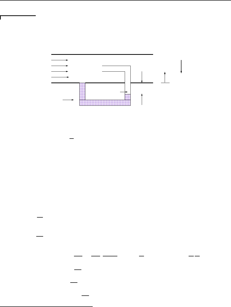
4.2. FLOW WITH AREA CHANGE 77
Example 4. 5
Pressure measurement in compressible flows
4
See Figure 4.5.
Air at
100 F
Mercury
8 inches
Stagnation
State "o"
Static
State "1"
z
g
Figure 4.5: Compressible pitot tube sketch
Given: Air at u = 750
ft
s
, Mercury manometer which reads a change in height of 8 inches.
Find: Static pressure of air in ps ia
Assume: Ideal gas b e havior for air
Analysis:
First consider the ma nometer which is governed by fluid statics. In fluid statics, there is no motion,
thus there are no viscous forces or fluid inertia; one thus has a balance between surface and body forces.
Consider the linear momentum equatio n:
ρ
dv
dt
= −∇P + ρ
Hg
g + ∇· τ (4.144)
0 = −∇P + ρ
Hg
g (4.145)
dP
dz
= ρ
Hg
g
z
(4.146)
P
1
− P
o
= ρ
Hg
g
z
(z
1
− z
o
) (4.147)
P
1
− P
o
=
845.9
lbm
ft
3
1
32.2
lbf s
2
ft lbm
−32.2
ft
s
2
(0 in −(−8 in))
1
12
ft
in
(4.148)
P
1
− P
o
= −56 3.9
lbf
ft
2
(4.149)
P
o
− P
1
= 563 .9
lbf
ft
2
(4.150)
P
o
= P
1
+ 563.9
lbf
ft
2
(4.151)
4
adopted from White, 9 .26, p. 584
CC BY-NC-ND. 28 October 2019, J. M. Powers.

78 CHAPTER 4. ONE-DIMENSIONAL COMPRESSIBLE FLOW
Now calculate the local Mach number
T
1
= 100 + 460 = 560 R (4.152)
M
1
=
u
1
√
γRT
1
(4.153)
M
1
=
750
ft
s
r
(1.4)
1, 717
ft
2
s
2
R
(560 R)
(4.154)
M
1
= 0.646 (4.155)
Isentropic flow relations relate stagnation to static properties, so for air
P
o
= P
1
1 +
1
5
M
2
1
3.5
(4.156)
P
o
= P
1
1 +
1
5
(0.646)
2
3.5
(4.157)
P
o
= 1.32 4P
1
(4.158)
Substituting from the measured pressure difference
P
1
+ 563.9
lbf
ft
2
= 1.32 4P
1
(4.159)
−0.324P
1
= −56 3.9
lbf
ft
2
(4.160)
P
1
=
−563.9
lbf
ft
2
−0.324
(4.161)
P
1
= 1, 740
lbf
ft
2
(4.162)
P
o
= (1.324)
1, 740
lbf
ft
2
= 2, 304
lbf
ft
2
(4.163)
P
1
=
1, 740
lbf
ft
2
1
12
ft
in
2
= 12.1 psia (4.164)
P
o
=
2, 304
lbf
ft
2
1
12
ft
in
2
= 16.0 psia (4.165)
What might one estimate if one did not account for compressibility effects? Assume one had the
same s tatic pressure and calculate what velocity one would predict.
First calculate the static density.
ρ
1
=
P
1
RT
1
(4.166)
ρ
1
=
1, 740
lbf
ft
2
1, 717
ft
2
s
2
R
(560 R)
32.2
ft lbm
lbf s
2
(4.167)
ρ
1
= 0.05 827
lbm
ft
3
(4.168)
CC BY-NC-ND. 28 October 2019, J. M. Powers.

4.2. FLOW WITH AREA CHANGE 79
One would then use an incompressible Berno ulli equation:
P
o
+
ρ (0)
2
2
= P
1
+
ρ
1
u
2
1
2
(4.169)
u
1
=
s
2 (P
o
− P
1
)
ρ
1
(4.170)
u
1
=
v
u
u
u
t
2
563.9
lbf
ft
2
0.05827
lbm
ft
3
32.2
ft lbm
lbf s
2
(4.171)
u
1
= 789 .4
ft
s
(4.172)
So the relative error in using the inc ompressible approximation would be
Error =
789.4 −750
750
= 5.3% (4.173)
Example 4. 6
Adiabatic Duct Flow
5
Given: Air flowing adiabatically through a duct. At section 1, u
1
= 400
ft
s
, T
1
= 200
◦
F, P
1
=
35 psia. Downstream u
2
= 1, 100
ft
s
, P
2
= 18 psia.
Find: M
2
, u
max
,
P
o2
P
o1
Assume: Calor ically perfect ideal gas, steady, one-dimensional flow
Analysis:
Some preliminaries :
T
1
= 200 + 460 = 660 R (4.174)
c
p
=
0.240
Btu
lbm R
779
ft lbf
Btu
32.17
lbm f t
lbf s
2
= 6, 015
ft
2
s
2
R
(4.175)
R =
53.34
ft lbf
lbm R
32.17
lbm f t
lbf s
2
= 1, 716
ft
2
s
2
R
(4.176)
(4.177)
Energy c onservation gives stagnation conditions at sta te 1
h
1
+
u
2
1
2
= h
o1
(4.178)
5
adopted from White’s 9.30, p. 585
CC BY-NC-ND. 28 October 2019, J. M. Powers.

80 CHAPTER 4. ONE-DIMENSIONAL COMPRESSIBLE FLOW
c
p
T
1
+
u
2
1
2
= c
p
T
o1
(4.179)
T
o1
= T
1
+
u
2
1
2c
p
(4.180)
T
o1
= 660 R +
400
ft
s
2
2
6, 015
ft
2
s
2
R
(4.181)
T
o1
= 673 R (4.182)
Note since in adiabatic flow h
o
is a constant, h
o2
= h
o1
and since ideal gas T
o2
= T
o1
So
T
o2
= 673 R (4.183)
T
2
= T
o2
−
u
2
2
2c
p
(4.184)
T
2
= 673 R −
1, 100
ft
s
2
2
6, 015
ft
2
s
2
R
(4.185)
T
2
= 572 R (4.186)
Calculate the Mach numbers:
c
1
=
p
γRT
1
(4.187)
c
1
=
s
1.4
1, 716
ft
2
s
2
R
(660 R) = 1, 259
ft
s
(4.188)
M
1
=
u
1
c
1
=
400
ft
s
1, 259
ft
s
= 0.31 8 (4.189)
c
2
=
p
γRT
2
(4.190)
c
2
=
s
1.4
1, 716
ft
2
s
2
R
(572 R) = 1, 173
ft
s
(4.191)
M
2
=
u
2
c
2
=
1, 100
ft
s
1, 173
ft
s
= 0.93 8 (4.192)
Since for CPIG air one has
P
P
o
=
1 +
1
5
M
2
−
7
2
(4.193)
P
o
= P
1 +
1
5
M
2
7
2
(4.194)
P
o1
= (35 psia)
1 +
1
5
0.318
2
7
2
= 37.5 4 psia (4.195)
P
o2
= (18 psia)
1 +
1
5
0.938
2
7
2
= 31.7 4 psia (4.196)
P
o2
P
o1
=
31.74 psia
37.54 psia
= 0.84 5 (4.197)
CC BY-NC-ND. 28 October 2019, J. M. Powers.

4.2. FLOW WITH AREA CHANGE 81
Stagnation pressure drop indicates that friction was pre sent. If one computed an entropy change one
would see an increase in entropy.
The maximum velocity is found by converting all the thermal energy to kinetic energy. Taking
zero thermal energy to correspond to abs olute zero (despite the fact that air would not be a gas at this
point) one could estimate
h
o
=
u
2
max
2
(4.198)
c
p
T
o
=
u
2
max
2
(4.199)
u
max
=
p
2c
p
T
o
(4.200)
u
max
=
s
2
6, 015
ft
2
s
2
R
(673 R) = 2, 845
ft
s
(4.201)
4.2.2 Sonic properties
Let “*” denote a property at the sonic state M
2
≡ 1
T
∗
T
o
=
1 +
γ − 1
2
1
2
−1
=
2
γ + 1
(4.202)
ρ
∗
ρ
o
=
1 +
γ − 1
2
1
2
−
1
γ−1
=
2
γ + 1
1
γ−1
(4.203)
P
∗
P
o
=
1 +
γ − 1
2
1
2
−
γ
γ−1
=
2
γ + 1
γ
γ−1
(4.204)
c
∗
c
o
=
1 +
γ − 1
2
1
2
−1/2
=
r
2
γ + 1
(4.205)
u
∗
= c
∗
=
p
γRT
∗
=
r
2γ
γ + 1
RT
o
(4.206)
If air γ = 7/5 and
T
∗
T
o
= 0.8333 (4.207)
ρ
∗
ρ
o
= 0.6339 (4.208)
P
∗
P
o
= 0.5283 (4.209)
c
∗
c
o
= 0.9129 (4.210)
CC BY-NC-ND. 28 October 2019, J. M. Powers.

82 CHAPTER 4. ONE-DIMENSIONAL COMPRESSIBLE FLOW
4.2.3 Effect of area change
Influence o f mass equation must be considered. So f ar only looked at energy has been
examined. In t he isentropic limit t he mass, momentum, and energy equation f or a CPIG
reduce t o
dρ
ρ
+
du
u
+
dA
A
= 0 ( 4.211)
ρudu + dP = 0 (4.212)
dP
P
= γ
dρ
ρ
(4.213)
Substitute energy then mass into momentum:
ρudu + γ
P
ρ
dρ = 0 (4.214)
ρudu + γ
P
ρ
−
ρ
u
du −
ρ
A
dA
= 0 ( 4.215)
du + γ
P
ρ
−
1
u
2
du −
1
uA
dA
= 0 ( 4.216)
du
1 −
γP/ρ
u
2
= γ
P
ρ
dA
uA
(4.217)
du
u
1 −
γP/ρ
u
2
=
γP/ρ
u
2
dA
A
(4.218)
du
u
1 −
1
M
2
=
1
M
2
dA
A
(4.219)
du
u
M
2
− 1
=
dA
A
(4.220)
du
u
=
1
M
2
− 1
dA
A
(4.221)
Figure 4.6 gives show the performance of a fluid in a variable area duct.
It is noted that
• equation singular when M
2
= 1
• if M
2
= 1, one needs dA = 0
• area minimum necessary to transition from subsonic to supersonic flow!!
• can be shown ar ea maximum not relevant
Consider A at a sonic state. From the mass equation:
ρuA = ρ
∗
u
∗
A
∗
(4.222)
CC BY-NC-ND. 28 October 2019, J. M. Powers.

4.2. FLOW WITH AREA CHANGE 83
Consider u > 0
Subsonic
Diffuser
Subsonic
Nozzle
Supersonic
Nozzle
Supersonic
Diffuser
dA > 0, M < 1 so
du < 0, flow slows down
dp > 0
2
dA < 0, M <1 so
du > 0, flow speeds up
dp < 0
2
dA < 0, M > 1 so
du < 0, flow slows down
dp > 0
2
dA > 0, M >1 so
du > 0, flow speeds up
dp < 0
2
Figure 4.6: Behavior of fluid in sub- and supersonic nozzles and diffusers
ρuA = ρ
∗
c
∗
A
∗
(4.223)
A
A
∗
=
ρ
∗
ρ
c
∗
1
u
, (4.224)
=
ρ
∗
ρ
p
γRT
∗
1
u
, (4.225)
=
ρ
∗
ρ
√
γRT
∗
√
γRT
√
γRT
u
(4.226)
=
ρ
∗
ρ
r
T
∗
T
1
M
, (4.227)
=
ρ
∗
ρ
o
ρ
o
ρ
r
T
∗
T
o
T
o
T
1
M
(4.228)
Substitute from earlier-developed relations and g et:
A
A
∗
=
1
M
2
γ + 1
1 +
γ − 1
2
M
2
1
2
γ+1
γ−1
(4.229)
Figure 4.7 shows the performance of a fluid in a variable area duct.
Note:
CC BY-NC-ND. 28 October 2019, J. M. Powers.

84 CHAPTER 4. ONE-DIMENSIONAL COMPRESSIBLE FLOW
0 0.5
1
1.5
2
2.5 3
M
1
2
3
4
5
6
A/A*
calorically perfect
ideal gas
R = 0.287 kJ/(kg K)
γ = 7/5
Figure 4.7: Area versus Mach number f or a calorically perfect ideal gas
•
A
A
∗
has a minimum value of 1 at M = 1
• For each
A
A∗
> 1, there exist two values of M
•
A
A
∗
→ ∞ as M → 0 or M → ∞
4.2.4 Choking
Consider ma ss flow rate variation with pressure difference
• small pressure difference gives small velocity, small mass flow
• as pressure difference grows, velocity and mass flow rate grow
• velocity is limited to sonic at a particular duct locat ion
• this provides fundamental restriction on mass flow rate
• can be proven rigorously that sonic conditio n gives maximum mass flow rate
˙m
max
= ρ
∗
u
∗
A
∗
(4.230)
if ideal gas: = ρ
o
2
γ + 1
1
γ−1
r
2γ
γ + 1
RT
o
A
∗
(4.231)
= ρ
o
2
γ + 1
1
γ−1
2
γ + 1
1/2
p
γRT
o
A
∗
(4.232)
= ρ
o
2
γ + 1
1
2
γ+1
γ−1
p
γRT
o
A
∗
(4.233)
A flow which has a maximum mass flow rate is known as choked flow. F lows will choke
at area minima in a duct.
CC BY-NC-ND. 28 October 2019, J. M. Powers.

4.2. FLOW WITH AREA CHANGE 85
Example 4. 7
Isentropic area change problem with choking
6
Given: Air with stagnation conditions P
o
= 200 kP a T
o
= 500 K flows through a throat to an exit
Mach number of 2.5. The desired mass flow is 3.0 kg/s,
Find: a) throat area, b) exit pre ssure, c) exit temperature, d) exit velocity, and e) exit area.
Assume: CPIG, isentropic flow, γ = 7/5
Analysis:
ρ
o
=
P
o
RT
o
=
200 kP a
(0.287 kJ/kg) (500 K)
= 1.394 kg/m
3
(4.234)
Since it necessarily flows through a sonic throa t:
˙m
max
= ρ
o
2
γ + 1
1
2
γ+1
γ−1
p
γRT
o
A
∗
(4.235)
A
∗
=
˙m
max
ρ
o
2
γ+1
1
2
γ+1
γ−1
√
γRT
o
(4.236)
=
3 kg/s
1.394
kg
m
3
(0.5787)
r
1.4
287
J
kg K
(500 K)
, (4.237)
= 0.00 8297 m
2
(4.238)
Since M
e
is known, use the isentropic relations to find other ex it conditions.
P
e
= P
o
1 +
γ − 1
2
M
2
e
−
γ
γ−1
, (4.239)
= (200 kP a )
1 +
1
5
2.5
2
−3.5
, (4.240)
= 11.7 1 kP a (4.241)
T
e
= T
o
1 +
γ − 1
2
M
2
e
−1
, (4.242)
= (500 K)
1 +
1
5
2.5
2
−1
, (4.243)
= 222 .2 K (4.244)
Note
ρ
e
=
P
e
RT
e
, (4.245)
=
11.71 kP a
0.287
kJ
kgK
(222.2 K)
, (4.24 6)
= 0.18 34
kg
m
3
(4.247)
6
adopted from White, Fluid Mechanics McGraw-Hill: New York, 1986 , p. 529, Ex. 9.5
CC BY-NC-ND. 28 October 2019, J. M. Powers.

86 CHAPTER 4. ONE-DIMENSIONAL COMPRESSIBLE FLOW
Now the exit velocity is simply
u
e
= M
e
c
e
= M
e
p
γRT
e
= 2.5
s
1.4
287
J
kg K
(222.2 K) = 747.0
m
s
(4.248)
Now determine the exit area:
A =
A
∗
M
e
2
γ + 1
1 +
γ − 1
2
M
2
e
1
2
γ+1
γ−1
(4.249)
=
0.008297 m
2
2.5
5
6
1 +
1
5
2.5
2
3
, (4.250)
= 70.0219 m
2
(4.251)
Example 4. 8
Discharge Problem
7
Given: Air in tank, P
o
= 700 kP a, T
o
= 20
◦
C, V = 1.5 m
3
. Thr oat area in converging nozzle of
0.65 cm
2
, exhausting to 1 atm environment
Find: Time for pressure in tank to decrease to 500 kP a.
Assume: CP I G, stagnation temperature cons tant (so small heat transfer to tank in time of opera-
tion)
Analysis:
First, T
o
= 20 + 273 = 293 K
Now check for choked flow! At the initial state
P
atm
P
o
=
101.3 kP a
700 kP a
= 0.145 (4.252)
But for air
P
∗
P
o
= 0.5283, so the flow must be choked at the exit and the ma ss flow is res tricted.
(Further expansion takes place outside the nozzle)
For choked flow one has
˙m
e
= ρ
o
2
γ + 1
1
2
γ+1
γ−1
p
γRT
o
A
∗
(4.253)
=
P
o
RT
o
2
γ + 1
1
2
γ+1
γ−1
p
γRT
o
A
∗
(4.254)
=
P
o
287
J
kg K
(293 K)
0.5787
s
1.4
287
J
kg K
(293 K)
0.65 cm
2
1
100
m
cm
2
(4.255)
= 1.53 48 × 10
−7
P
o
(4.256)
7
from White, 9.33,35
CC BY-NC-ND. 28 October 2019, J. M. Powers.

4.3. NORMAL SHOCK WAVES 87
Now mass conservation gives
d
dt
m
cv
= − ˙m
e
(4.257)
d
dt
(ρ
o
V ) = − ˙m
e
(4.258)
d
dt
P
o
RT
o
V
= − ˙m
e
(4.259)
dP
o
dt
= −
RT
o
V
˙m
e
(4.260)
dP
o
dt
= −
287
J
kg K
(293 K)
1.5 m
3
1.5348 ×10
−7
P
o
(4.261)
dP
o
dt
= −0.0 08604P
o
(4.262)
P
o
= A exp (−0.008604t) (4.2 63)
Use initial value of P
o
to fix the constant A so
P
o
= 700 exp (−0.008604t) (4.2 64)
When doe s P
o
= 500 kP a?
500 = 700 exp (−0.008604t) ln
500
700
= −0.008604t (4.265)
t = −
1
0.008604
ln
500
700
= 39.1 s (4.266)
4.3 Normal shock waves
This section will develop relations for normal shock waves in fluids with general equations of
state. It will be specialized to calorically perfect ideal gases to illustrate the general features
of the waves.
Assumptions for this section
• one-dimensional flow
• steady flow
• no area change
• viscous effects and wall friction do not have time to influence flow
• heat conduction and wall heat transfer do not have time to influence flow
CC BY-NC-ND. 28 October 2019, J. M. Powers.

88 CHAPTER 4. ONE-DIMENSIONAL COMPRESSIBLE FLOW
Steady Frame
x
u = - D
P
1
ρ
1
u
2
P
2
ρ
2
Laboratory Frame
v = 0
P
1
ρ
1
v = v
2
P
2
ρ
2
v
p
= v
2
D
u = v - D; v = u + D
x = x* - D t; x* = x + D t
x*
Figure 4.8: Normal shock sketch
The piston problem as sketched in Figure 4.8 will be considered.
Physical problem:
• Drive piston with known velocity v
p
into fluid at rest (v
1
= 0) with known properties,
P
1
, ρ
1
in the x
∗
laborato r y frame
• Determine disturbance speed D
• Determine disturbance properties v
2
, P
2
, ρ
2
• in this frame of reference unsteady problem
Transformed Problem:
• use Galilean transformatio n x = x
∗
−Dt, u = v −D to transfor m to the frame in which
the wave is at rest, therefore rending the problem steady in this fr ame
• solve as though D is known to get downstream “2” conditio ns: u
2
(D), P
2
(D), ...
• invert to solve for D as function of u
2
, t he transfor med piston velocity: D(u
2
)
• back transform to get all variables as function of v
2
, the labo ratory piston velocity:
D(v
2
), P
2
(v
2
), ρ
2
(v
2
), ...
4.3.1 Governing equations
Under these assumptions the conservat ion principles in conservative form and equation of
state are in the steady frame as fo llows:
d
dx
(ρu) = 0 (4.267)
d
dx
ρu
2
+ P
= 0 (4.268)
CC BY-NC-ND. 28 October 2019, J. M. Powers.

4.3. NORMAL SHOCK WAVES 89
d
dx
ρu
h +
u
2
2
= 0 (4.269)
h = h(P, ρ) (4.270)
Upstream conditions are ρ = ρ
1
, P = P
1
, u = −D. With knowledge of the equation of
state, one gets h = h
1
. Integrating the equations from upstream to state “2” gives:
ρ
2
u
2
= −ρ
1
D (4.271)
ρ
2
u
2
2
+ P
2
= ρ
1
D
2
+ P
1
(4.272)
h
2
+
u
2
2
2
= h
1
+
D
2
2
(4.273)
h
2
= h(P
2
, ρ
2
) (4.274)
4.3.2 Rayleigh line
Work on the momentum equation:
P
2
= P
1
+ ρ
1
D
2
− ρ
2
u
2
2
(4.275)
P
2
= P
1
+
ρ
2
1
D
2
ρ
1
−
ρ
2
2
u
2
2
ρ
2
(4.276)
Since mass gives ρ
2
2
u
2
2
= ρ
2
1
D
2
one gets an equation for the Rayleigh Line, a line in (P,
1
ρ
)
space:
P
2
= P
1
+ ρ
2
1
D
2
1
ρ
1
−
1
ρ
2
(4.277)
Note:
• Rayleigh line passes through ambient state
• Rayleigh line has negative slope
• magnitude of slope proportional t o square of wave speed
• independent of state and energy equations
4.3.3 Hugoniot curve
Operate on the energy equation, using both mass and moment um to eliminate velocity. First
eliminate u
2
via the mass equation:
CC BY-NC-ND. 28 October 2019, J. M. Powers.

90 CHAPTER 4. ONE-DIMENSIONAL COMPRESSIBLE FLOW
h
2
+
u
2
2
2
= h
1
+
D
2
2
(4.278)
h
2
+
1
2
ρ
1
D
ρ
2
2
= h
1
+
D
2
2
(4.279)
h
2
− h
1
+
D
2
2
ρ
1
ρ
2
2
− 1
!
= 0 (4.280)
h
2
− h
1
+
D
2
2
ρ
2
1
− ρ
2
2
ρ
2
2
= 0 (4.281)
h
2
− h
1
+
D
2
2
(ρ
1
− ρ
2
) (ρ
1
+ ρ
2
)
ρ
2
2
= 0 (4.282)
Now use t he Rayleigh line to eliminate D
2
:
D
2
= (P
2
− P
1
)
1
ρ
2
1
1
ρ
1
−
1
ρ
2
−1
(4.283)
D
2
= (P
2
− P
1
)
1
ρ
2
1
ρ
2
− ρ
1
ρ
1
ρ
2
−1
(4.284)
D
2
= (P
2
− P
1
)
1
ρ
2
1
ρ
1
ρ
2
ρ
2
− ρ
1
(4.285)
so the energy equation becomes
h
2
− h
1
+
1
2
(P
2
− P
1
)
1
ρ
2
1
ρ
1
ρ
2
ρ
2
− ρ
1
(ρ
1
− ρ
2
) (ρ
1
+ ρ
2
)
ρ
2
2
= 0 (4.286)
h
2
− h
1
−
1
2
(P
2
− P
1
)
1
ρ
1
ρ
1
+ ρ
2
ρ
2
= 0 (4.287)
h
2
− h
1
−
1
2
(P
2
− P
1
)
1
ρ
2
+
1
ρ
1
= 0 (4.288)
(4.289)
Solving finally for the enthalpy difference, one finds
h
2
− h
1
= (P
2
− P
1
)
1
2
1
ρ
2
+
1
ρ
1
(4.290)
This equation is the Hugoniot equation.
• enthalpy change equals pressure difference times mean volume
• independent of wave speed D and velocity u
2
• independent of equation of state
CC BY-NC-ND. 28 October 2019, J. M. Powers.

4.3. NORMAL SHOCK WAVES 91
4.3.4 Solution procedure for general equations of state
The shocked state can be determined by the following procedure:
• specify and equation of state h(P, ρ)
• substitute the equation of state into the Hugoniot to get a second relation between P
2
and ρ
2
.
• use the Rayleigh line to eliminate P
2
in the Hugoniot so that the Hugoniot is a single
equation in ρ
2
• solve for ρ
2
as functions of “1 ” and D
• back substitute to solve for P
2
, u
2
, h
2
, T
2
as functions of “1” and D
• invert to find D as function of “1” state and u
2
• back transform to laboratory frame to get D as function of “1” state and piston velocity
v
2
= v
p
4.3.5 Calorically perfect ideal gas solutions
Follow this procedure for the special case of a calorically perfect ideal gas.
h = c
p
(T −T
o
) + h
o
(4.291)
P = ρR T (4.292)
so
h = c
p
P
Rρ
−
P
o
Rρ
o
+ h
o
(4.293)
h =
c
p
R
P
ρ
−
P
o
ρ
o
+ h
o
(4.294)
h =
c
p
c
p
− c
v
P
ρ
−
P
o
ρ
o
+ h
o
(4.295)
h =
γ
γ − 1
P
ρ
−
P
o
ρ
o
+ h
o
(4.296)
Evaluate at states 1 and 2 and substitute into Hugoniot:
γ
γ − 1
P
2
ρ
2
−
P
o
ρ
o
+ h
o
−
γ
γ − 1
P
1
ρ
1
−
P
o
ρ
o
+ h
o
= (P
2
− P
1
)
1
2
1
ρ
2
+
1
ρ
1
CC BY-NC-ND. 28 October 2019, J. M. Powers.

92 CHAPTER 4. ONE-DIMENSIONAL COMPRESSIBLE FLOW
γ
γ − 1
P
2
ρ
2
−
P
1
ρ
1
− (P
2
− P
1
)
1
2
1
ρ
2
+
1
ρ
1
= 0
P
2
γ
γ − 1
1
ρ
2
−
1
2ρ
2
−
1
2ρ
1
− P
1
γ
γ − 1
1
ρ
1
−
1
2ρ
2
−
1
2ρ
1
= 0
P
2
γ + 1
2 (γ − 1)
1
ρ
2
−
1
2ρ
1
− P
1
γ + 1
2 (γ − 1)
1
ρ
1
−
1
2ρ
2
= 0
P
2
γ + 1
γ − 1
1
ρ
2
−
1
ρ
1
− P
1
γ + 1
γ − 1
1
ρ
1
−
1
ρ
2
= 0
P
2
= P
1
γ+1
γ−1
1
ρ
1
−
1
ρ
2
γ+1
γ−1
1
ρ
2
−
1
ρ
1
• a hyperbola in (P,
1
ρ
) space
•
1
ρ
2
→
γ−1
γ+1
1
ρ
1
causes P
2
→ ∞, note for γ = 1.4, ρ
2
→ 6ρ
1
for infinite pressure
• as
1
ρ
2
→ ∞, P
2
→ −P
1
γ−1
γ+1
, note negative pressure, not physical here
The Rayleigh line and Hugonio t curves are sketched in Figure 4.9.
2
3 4
5
6
7
100
200
300
400
500
1/ρ (kg/m )
3
P (kPa)
1/ρ
1
1/ρ
2
P
1
P
2
initial state
excluded zone
slope of Rayleigh line < 0
excluded zone, 2nd law violation
Hugoniot,
from energy
Rayleigh line, slope ~ D
from mass and momentum
2
1/ρ = (γ-1) 1
(γ+1) ρ
min
1
-(γ-1) P
1
γ+1
excluded zone, negative pressure
shocked state
excluded
zone,
1/ρ < 1/ρ
min
Figure 4.9: Rayleigh line and Hugoniot curve.
Note:
• intersections of the two curves are solutions to the equations
• the ambient state “1” is o ne solution
CC BY-NC-ND. 28 October 2019, J. M. Powers.

4.3. NORMAL SHOCK WAVES 93
• the other solutio n “2” is known as t he shock solution
• shock solution has higher pressure a nd higher density
• higher wave speed implies higher pressure and higher density
• a minimum wavespeed exists
– occurs when Rayleigh line tangent to Hugoniot
– occurs for very small pressure changes
– corresponds t o a sonic wave speed
– disturbances a r e acoustic
• if pressure increases, can be shown entropy increases
• if pressure decreases ( wave speed less than sonic), entropy decreases; this is non-
physical
Substitute Rayleigh line into Hugoniot to get single equation for ρ
2
P
1
+ ρ
2
1
D
2
1
ρ
1
−
1
ρ
2
= P
1
γ+1
γ−1
1
ρ
1
−
1
ρ
2
γ+1
γ−1
1
ρ
2
−
1
ρ
1
(4.297)
This equation is quadratic in
1
ρ
2
and factorizable. Use computer algebra to solve and get
two solutions, one ambient
1
ρ
2
=
1
ρ
1
and one shocked solution:
1
ρ
2
=
1
ρ
1
γ − 1
γ + 1
1 +
2γ
(γ − 1) D
2
P
1
ρ
1
(4.298)
The shocked density ρ
2
is plotted against wave speed D for CPIG air in Figure 4.10.
Note
• density solution allows allows all wave speeds 0 < D < ∞
• plot range, however, is c
1
< D < ∞
• Rayleigh line and Hugoniot show D ≥ c
1
• solution for D = D(v
p
), to be shown, rigorously shows D ≥ c
1
• strong shock limit: D
2
→ ∞, ρ
2
→
γ+1
γ−1
• acoustic limit: D
2
→ γ
P
1
ρ
1
, ρ
2
→ ρ
1
• non-physical limit: D
2
→ 0, ρ
2
→ 0
CC BY-NC-ND. 28 October 2019, J. M. Powers.

94 CHAPTER 4. ONE-DIMENSIONAL COMPRESSIBLE FLOW
strong
shock
limit
calorically perfect
ideal air
γ = 7/5
R = 0.287 kJ/(kg K)
exact
solution
D = D
min
= c
1
500 1000 1500 2000 2500 3000
D (m/s
)
1
2
3
4
5
6
7
ρ
2
(kg/m
3
)
Figure 4.10: Shock density vs. shock wave speed for calorically perfect ideal air.
Back substitute into Rayleigh line and mass conservation to solve for the shocked pressure
and the fluid velocity in the shocked wave frame:
P
2
=
2
γ + 1
ρ
1
D
2
−
γ − 1
γ + 1
P
1
(4.299)
u
2
= −D
γ − 1
γ + 1
1 +
2γ
(γ − 1) D
2
P
1
ρ
1
(4.300)
The shocked pressure P
2
is plotted against wave speed D for CPIG air in Figure 4.11
including both the exact solution and the solution in the strong shock limit. Note for these
parameters, the results a re indistinguishable.
calorically perfect
ideal air
γ = 7/5
R = 0.287 kJ/(kg K)
exact
solution and
strong shock limit
ambient =
100000 Pa
D = D
min
= c
1
500 1000 1500 2000 2500 3000
D (m/s
)
6
2. 10
6
4. 10
6
6. 10
6
8. 10
P
2
(Pa)
x
x
x
x
Figure 4.11: Shock pressure vs. shock wave speed f or calorically perfect ideal air.
The shocked wave frame fluid par ticle velocity u
2
is plotted against wave speed D for
CPIG air in Figure 4.12.
CC BY-NC-ND. 28 October 2019, J. M. Powers.

4.3. NORMAL SHOCK WAVES 95
strong
shock
limit
γ = 7/5
R = 0.287 kJ/(kg K)
exact
solution
u
1
= - c
1
D = D
min
= c
1
500 1000 1500 2000 2500 3000
D (m/s
)
-500
-400
-300
-200
-100
u
2
(m/s)
calorically perfect
ideal air
Figure 4.12: Shock wave frame fluid particle velocity vs. shock wave speed for calorically
perfect ideal a ir.
The shocked wave frame fluid pa rticle velocity M
2
2
=
ρ
2
u
2
2
γP
2
is plotted against wave speed
D for CPIG air in F igure 4 .13.
calorically perfect
ideal air
γ = 7/5
R = 0.287 kJ/(kg K)
exact
solution
strong
shock
limit
D = D
min
= c
1
M
2
2
= 1
0 500 1000 1500 2000 2500 3000
D (m/s
)
0.2
0.4
0.6
0.8
1
M
2
2
Figure 4.13: Mach number squared of shocked fluid particle vs. shock wave speed for calor-
ically perfect ideal a ir .
Exercise: For t he conditions shown in the plot of M
2
2
vs. D do the detailed calculations
to demonstrate the plot is correct.
Note in the steady frame that
• The Mach number of the undisturbed flow is (and must be) > 1: supersonic
• The Mach number of the shocked flow is (and must be) < 1 : subson i c
CC BY-NC-ND. 28 October 2019, J. M. Powers.

96 CHAPTER 4. ONE-DIMENSIONAL COMPRESSIBLE FLOW
Transform back to the laboratory frame u = v − D:
v
2
− D = −D
γ − 1
γ + 1
1 +
2γ
(γ − 1) D
2
P
1
ρ
1
(4.301)
v
2
= D −D
γ − 1
γ + 1
1 +
2γ
(γ − 1) D
2
P
1
ρ
1
(4.302)
Manipulate the above equation and solve the resulting quadra tic equation for D and get
D =
γ + 1
4
v
2
±
s
γP
1
ρ
1
+ v
2
2
γ + 1
4
2
(4.303)
Now if v
2
> 0, one expects D > 0 so take positive root, also set velocity equal piston
velocity v
2
= v
p
D =
γ + 1
4
v
p
+
s
γP
1
ρ
1
+ v
2
p
γ + 1
4
2
(4.304)
Note:
• acoustic limit: as v
p
→ 0, D → c
1
; the shock speed approaches the sound speed
• strong shock limit: as v
p
→ ∞, D →
γ+1
2
v
p
The shock speed D is plotted against piston velocity v
p
for CPIG air in Figure 4.14. Both
the exact solution and strong shock limit are shown.
200 400 600 800 1000
v
p
(m/s
)
200
400
600
800
1000
1200
D (m/s)
exact
solution
acoustic
limit,
D c
1
calorically perfect
ideal air
γ = 7/5
R = 0.287 kJ/(kg K)
strong
shock
limit
Figure 4.14: Shock speed vs. piston velocity for calorically perfect ideal air.
If the Mach number of the shock is defined as
M
s
≡
D
c
1
(4.305)
CC BY-NC-ND. 28 October 2019, J. M. Powers.
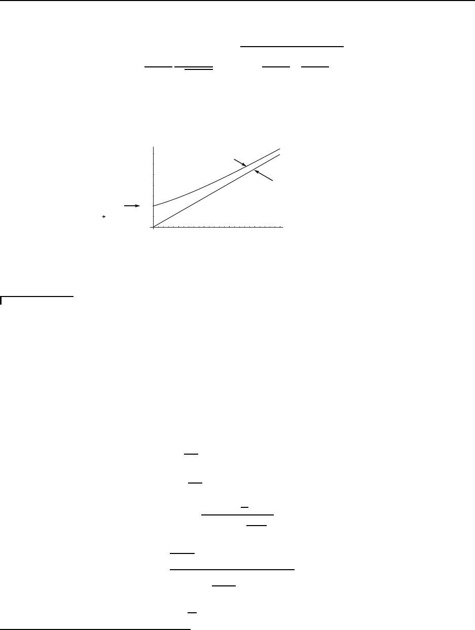
4.3. NORMAL SHOCK WAVES 97
one g ets
M
s
=
γ + 1
4
v
p
√
γRT
1
+
s
1 +
v
2
p
γRT
1
γ + 1
4
2
(4.306)
The shock Mach number M
s
is plotted against piston velocity v
p
for CPIG air in Figure
4.15. Both the exact solution and strong shock limit are shown.
200 400 600 800 1000
v
p
(m/s)
0.5
1
1.5
2
2
.5
3
3.5
M
s
strong
shock
limit
exact
solution
acoustic
limit,
M
s
1
calorically perfect
ideal air
γ = 7/5
R = 0.287 kJ/(kg K)
Figure 4.15: Shock Mach number vs. piston velocity for calorically perfect ideal air
Example 4. 9
Normal shock problem
8
Given: Air flowing through normal shock. Upstream u
1
= 600 m /s, T
o1
= 500 K, P
o1
= 700 kP a.
Find: Downstream conditions M
2
, u
2
, T
2
, P
2
, P
o2
and s
2
− s
1
.
Assume: calorically perfect ideal gas
Analysis:
First get all loca l unshocked conditions.
T
o1
= T
1
+
u
2
1
2c
p
(4.307)
T
1
= T
o1
−
u
2
1
2c
p
(4.308)
T
1
= 500 K −
600
m
s
2
2
1004.5
J
kg K
, (4.309)
= 320 .81 K (4.310)
c
1
=
p
γRT
1
, (4.311)
=
s
1.4
287
J
kg K
(320.81 K), (4.312)
= 359 .0
m
s
(4.313)
8
adopted from White’s 9.46, p. 58 6
CC BY-NC-ND. 28 October 2019, J. M. Powers.

98 CHAPTER 4. ONE-DIMENSIONAL COMPRESSIBLE FLOW
M
1
=
u
1
c
1
, (4.314)
=
600
m
s
359.0
m
s
, (4.315)
= 1.67 1 (4.316)
P
1
= P
o1
1 +
1
5
M
2
1
−3.5
, (4.317)
= (700 kP a )
1 +
1
5
(1.671)
2
−3.5
, (4.318)
= 148 .1 kP a (4.319)
ρ
1
=
P
1
RT
1
, (4.320)
=
148.1 kP a
0.287
kJ
kg K
(320.81 K)
, (4.321)
= 1.60 9
kg
m
3
(4.322)
A
1
A
1∗
=
1
M
1
2
γ + 1
1 +
γ − 1
2
M
2
1
1
2
γ+1
γ−1
(4.323)
=
1
1.671
2
1.4 + 1
1 +
1.4 −1
2
1.671
2
1
2
1.4+1
1.4−1
, (4.324)
= 1.31 1 (4.325)
Now in this case it is fortunate because the incoming velocity D = 6 00
m
s
is known. Note that the
shock density only depends on D
2
, so one can be a little s loppy here with sign. Solve for the shocked
state:
1
ρ
2
=
1
ρ
1
γ − 1
γ + 1
1 +
2γ
(γ − 1) D
2
P
1
ρ
1
(4.326)
1
ρ
2
=
1
1.609
kg
m
3
1.4 −1
1.4 + 1
1 +
2 (1.4 )
(1.4 −1 )
600
m
s
2
148, 100 P a
1.609
kg
m
3
!
(4.327)
= 0.28 90
m
3
kg
(4.328)
ρ
2
=
1
0.2890
m
3
kg
, (4.329)
= 3.46 1
kg
m
3
(4.330)
Now a variety of equatio ns can be used to determine the remaining state variables. Mass gives u
2
:
ρ
2
u
2
= ρ
1
u
1
(4.331)
u
2
=
ρ
1
u
1
ρ
2
, (4.332)
=
1.609
kg
m
3
600
m
s
3.461
kg
m
3
, (4.333)
CC BY-NC-ND. 28 October 2019, J. M. Powers.

4.3. NORMAL SHOCK WAVES 99
= 278.9
m
s
. (4.334)
Momentum gives P
2
P
2
+ ρ
2
u
2
2
= P
1
+ ρ
1
u
2
1
(4.335)
P
2
= P
1
+ ρ
1
u
2
1
− ρ
2
u
2
2
(4.336)
P
2
= 148 , 100 P a +
1.609
kg
m
3
600
m
s
2
−
3.461
kg
m
3
278.9
m
s
2
(4.337)
P
2
= 458, 125 P a = 458 kP a (4.338)
Remaining assorted variables are straightforward:
T
2
=
P
2
ρ
2
R
(4.339)
=
458, 125 P a
3.461
kg
m
3
287
J
kg K
, (4.340)
= 461.2 K (4.341)
c
2
=
p
γRT
2
, (4.342)
=
s
1.4
287
J
kg K
(461.2 K), (4.343)
= 430.5
m
s
(4.344)
M
2
=
u
2
c
2
, (4.345)
=
278.9
m
s
430.5
m
s
, (4.346)
= 0.648 (4.347)
T
o2
= T
2
1 +
1
5
M
2
2
, (4.348)
= 461.2 K
1 +
1
5
0.648
2
(4.349)
= 500 K unchanged as re quired (4.350)
P
o2
= P
2
1 +
1
5
M
2
2
3.5
, (4.351)
= 458 kP a
1 +
1
5
0.648
2
3.5
(4.352)
= 607.4 kP a dropped from unshocked state (4.353)
s
2
− s
1
= c
p
ln
T
2
T
1
− R ln
P
2
P
1
(4.354)
= 1004.5
J
kg K
ln
461.2 K
320.81 K
− 287
J
kg K
ln
458 kP a
148.1 kP a
(4.355)
= 364.6 −324.0, (4.356)
= 40.6
J
kg K
(4.357)
A
2
A
2∗
=
1
M
2
2
γ + 1
1 +
γ − 1
2
M
2
2
1
2
γ+1
γ−1
(4.358)
CC BY-NC-ND. 28 October 2019, J. M. Powers.

100 CHAPTER 4. ONE-DIMENSIONAL COMPRESSIBLE FLOW
=
1
0.648
2
1.4 + 1
1 +
1.4 −1
2
0.648
2
1
2
1.4+1
1.4−1
, (4.359)
= 1.966. (4.360)
Since A
2
= A
1
= A,
A
2
A
2∗
=
A
A
1∗
A
A
2∗
=
1.311
1.966
= 0.667 (4.36 1)
Note the entropy incre ased despite not including a ny entropy-generating mechanisms in this model.
Why? First, the differential equations themselves required the assumption of continuous differentiable
functions. Our shock violates this. When one returns to the more fundamental control volume forms,
it can be shown tha t the entropy-generating mechanism returns. Fro m a continuum point o f view, one
can also show that the neglected terms, that momentum and energy diffusion, actually give rise to a
smeared shock. These mechanisms generate just enough entro py to satisfy the entropy jump which was
just calculated. Just as with Burger’s equation and the kinematic wave equation, the jumps are the
same, diffusion s imply gives a wave thickness.
Example 4. 10
Piston Problem
Given: A piston moving at v
p
= 1, 000
m
s
is driven into Helium which is at rest in the ambient
state at a pressure of P
1
= 10 kP a, T
1
= 50 K.
Find: The shock speed and post shock state.
Assume: Helium is calorically perfect and ideal
Analysis: For Helium,
γ = 1.667 (4.362)
R = 2077
J
kg K
(4.363)
c
p
=
γR
γ − 1
, (4.364)
=
1.667
2, 077
J
kg K
1.667 −1
, (4.365)
= 5, 192.5
J
kg K
. (4.366)
Ambient density
ρ
1
=
P
1
RT
1
, (4.367)
=
10, 000 P a
2, 077
J
kg K
(50 K)
, (4.368)
CC BY-NC-ND. 28 October 2019, J. M. Powers.

4.3. NORMAL SHOCK WAVES 101
= 0.09 63
kg
m
3
(4.369)
c
1
=
p
γRT
1
, (4.370)
=
s
1.667
2, 077
J
kg K
(50 K), (4.371)
= 416 .0
m
s
(4.372)
Now the wave spee d D one gets from
D =
γ + 1
4
v
p
+
s
γP
1
ρ
1
+ v
2
p
γ + 1
4
2
(4.373)
=
1.667 + 1
4
1, 000
m
s
+
v
u
u
t
1.667 (10, 000 P a)
0.0963
kg
m
3
+
1, 000
m
s
2
1.667 + 1
4
2
(4.374)
= 666 .7 + 785.8, (4.375)
= 1, 452.5
m
s
(4.376)
Strong shock limit is appropriate here as a quick check:
D ∼
γ + 1
2
v
p
=
1.667 + 1
2
1, 000
m
s
= 1, 333.3
m
s
(4.377)
P
2
=
2
γ + 1
ρ
1
D
2
−
γ − 1
γ + 1
P
1
(4.378)
=
2
1.667 + 1
0.0963
kg
m
3
1, 452.5
m
s
2
−
1.667 −1
1.667 + 1
(10, 0 00 P a) (4.379)
= 152 , 377 − 2, 500, (4.380)
= 149 , 877 P a = 150 kP a (4.381)
ρ
2
u
2
= ρ
1
u
1
(4.382)
ρ
2
(v
2
− D) = ρ
1
(v
1
− D) (4.383)
ρ
2
(v
p
− D) = ρ
1
(0 −D) (4.384)
ρ
2
=
−ρ
1
D
v
p
− D
(4.385)
=
−
0.0963
kg
m
3
1, 452.5
m
s
1, 000
m
s
− 1, 452.5
m
s
, (4.386)
= 0.30 9
kg
m
3
(4.387)
T
2
=
P
2
ρ
2
R
(4.388)
=
149, 877 P a
0.309
kg
m
3
2, 077
J
kg K
, (4.389)
= 233 .5 K (4.390)
CC BY-NC-ND. 28 October 2019, J. M. Powers.

102 CHAPTER 4. ONE-DIMENSIONAL COMPRESSIBLE FLOW
4.3.6 Acous tic limit
Consider t hat state 2 is a small perturbation of state 1 so that
ρ
2
= ρ
1
+ ∆ρ (4.391)
u
2
= u
1
+ ∆u
1
(4.392)
P
2
= P
1
+ ∆P (4.393)
Substituting into the normal shock equations, one gets
(ρ
1
+ ∆ρ) (u
1
+ ∆u) = ρ
1
u
1
(4.394)
(ρ
1
+ ∆ρ) (u
1
+ ∆u)
2
+ (P
1
+ ∆P ) = ρ
1
u
1
2
+ P
1
(4.395)
γ
γ − 1
P
1
+ ∆P
ρ
1
+ ∆ρ
+
1
2
(u
1
+ ∆u)
2
=
γ
γ − 1
P
1
ρ
1
+
1
2
u
1
2
(4.396)
Expanding, one gets
ρ
1
u
1
+ ˜u
1
(∆ρ) + ρ
1
(∆u) + (∆ρ) (∆u) = ρ
1
u
1
ρ
1
u
1
2
+ 2ρ
1
u
1
(∆u) + u
1
2
(∆ρ) + ρ
1
(∆u)
2
+ 2u
1
(∆u) (∆ρ) + (∆ρ) (∆u)
2
+ (P
1
+ ∆P ) = ρ
1
u
1
2
+ P
1
γ
γ − 1
P
1
ρ
1
+
1
ρ
1
∆P −
P
1
ρ
2
1
∆ρ + ...
+
1
2
u
1
2
+ 2u
1
(∆u) + (∆u)
2
=
γ
γ − 1
P
1
ρ
1
+
1
2
u
1
2
Subtracting the base stat e and eliminating products of small quantities yields
u
1
(∆ρ) + ρ
1
(∆u) = 0 (4.397)
2ρ
1
u
1
(∆u) + u
1
2
(∆ρ) + ∆P = 0 ( 4.398)
γ
γ − 1
1
ρ
1
∆P −
P
1
ρ
2
1
∆ρ
+ u
1
(∆u) = 0 (4.399)
In matr ix form this is
u
1
ρ
1
0
u
1
2
2ρ
1
u
1
1
−
γ
γ−1
P
1
ρ
2
1
u
1
γ
γ−1
1
ρ
1
∆ρ
∆u
∆P
=
0
0
0
(4.400)
As the r ight hand side is zero, the determinant must be zero and there must be a linear
dependency of the solution. First check the determinant:
CC BY-NC-ND. 28 October 2019, J. M. Powers.

4.3. NORMAL SHOCK WAVES 103
u
1
2γ
γ − 1
u
1
− u
1
− ρ
1
γ
γ − 1
u
1
2
ρ
1
+
γ
γ − 1
P
1
ρ
2
1
= 0 (4.401)
u
1
2
γ − 1
(2γ − (γ − 1)) −
1
γ − 1
γ u
1
2
+ γ
P
1
ρ
1
= 0 (4.402)
u
1
2
(γ + 1) −
γ u
1
2
+ γ
P
1
ρ
1
= 0 (4.403)
u
1
2
= γ
P
1
ρ
1
= c
2
1
(4.404)
So the velocity is necessarily sonic for a small disturbance!
Take ∆u to be known and solve a resulting 2 × 2 system:
u
1
0
−
γ
γ−1
P
1
ρ
2
1
γ
γ−1
1
ρ
1
∆ρ
∆P
=
−ρ
1
∆u
−u
1
∆u
(4.405)
Solving yields
∆ρ = −
ρ
1
∆u
q
γ
P
1
ρ
1
(4.406)
∆P = −ρ
1
s
γ
P
1
ρ
1
∆u (4.407)
4.3.7 Non-ideal gas solutions
Non-ideal effects are important
• near the critical point
• for strong shocks
Some ot her points:
• qualitative trends the same as fo r ideal gases
• analysis is much more alg ebraically complicated
• extraneous solutions o ften arise which must be discarded
CC BY-NC-ND. 28 October 2019, J. M. Powers.

104 CHAPTER 4. ONE-DIMENSIONAL COMPRESSIBLE FLOW
Example 4. 11
Shock in van der Waals gas
Given: Shock wave D = 500
m
s
propagating into N
2
at rest at T
1
= 125 K, P
1
= 2 M P a.
Find: Shocked state
Assume: van der Waals equation of state accurately models gas behavior, specific heat constant.
Analysis:
First, some data for N
2
are needed. At P
1
= 2 M P a, N
2
has a boiling point of 115.5 K, so
the material is in the g as phase but very near the vapor dome. R = 296.8
J
kg K
, c
v
= 744.8
J
kg K
,
T
c
= 126.2 K, P
c
= 3, 390, 000 P a.
Since the material is near the vapor dome, the van der Waals equation may give a good first
correction for non-ideal e ffects.
P =
RT
v − b
−
a
v
2
(4.408)
P =
RT
1
ρ
− b
− aρ
2
(4.409)
P =
ρRT
1 −bρ
− aρ
2
(4.410)
As derived earlier, the corresponding caloric eq uation of state is
e(T, v) = e
o
+
Z
T
T
o
c
v
(
ˆ
T )d
ˆ
T + a
1
v
o
−
1
v
(4.411)
Taking c
v
constant and exchanging v for ρ gives
e(T, ρ) = e
o
+ c
v
(T − T
o
) + a (ρ
o
− ρ) (4.412)
Eliminating T in favor of P then gives
e(P, ρ) = e
o
+ c
v
P + aρ
2
(1 − bρ)
ρR
− T
o
!
+ a (ρ
o
− ρ) (4.413)
and in terms of h = e + P/ρ:
h(P, ρ) = e
o
+ c
v
P + aρ
2
(1 −bρ)
ρR
− T
o
!
+ a (ρ
o
− ρ) +
P
ρ
(4.414)
and h
2
− h
1
allows cancellation of the “o” state so that
h
2
− h
1
= c
v
P
2
+ aρ
2
2
(1 −bρ
2
)
ρ
2
R
−
P
1
+ aρ
2
1
(1 −bρ
1
)
ρ
1
R
!
− a (ρ
2
− ρ
1
) +
P
2
ρ
2
−
P
1
ρ
1
(4.415)
CC BY-NC-ND. 28 October 2019, J. M. Powers.

4.3. NORMAL SHOCK WAVES 105
The constants a and b are fixed so that an isotherm passing throug h the critical point, P = P
c
, T =
T
c
, passes thro ugh with
∂P
∂v
T
= 0 and
∂
2
P
∂v
2
T
= 0 A standard analysis
9
yields
a =
27
64
R
2
T
2
c
P
c
, (4.416)
=
27
64
296.8
J
kg K
2
(126.2 K)
2
3, 390, 000 P a
, (4.417)
= 174 .6
P a m
6
kg
2
(4.418)
b =
RT
c
8P
c
, (4.419)
=
296.8
J
kg K
(126.2 K)
8 (3, 390, 0 00 P a)
, (4.420)
= 0.00 138
m
3
kg
(4.421)
Find the ambient density.
2, 000, 000 P a =
ρ
1
296.8
J
kg K
(125 K)
1 −
0.00138
m
3
kg
ρ
1
−
174.6
P a m
6
kg
2
ρ
2
1
(4.422)
Three solutions (from computer algebra):
ρ
1
= 69.0 926
kg
m
3
physical (4.423)
ρ
1
= (327.773 + 112.702 i)
kg
m
3
non-physical (4.424)
ρ
1
= (327.773 + 112.702 i)
kg
m
3
non-physical (4.425)
Tabular da ta from experiments gives ρ
1
= 71.28
kg
m
3
, error = (71.28−69.09)/71.28 = 3%, so it s e ems the
first root is the physical root. Note that the van der Waals prediction is a significant improvement over
the ideal gas law which gives ρ
1
=
P
1
RT
1
=
2,000,000
296.8×125
= 53.91
kg
m
3
, error = (71.28 −53.91)/71.28 = 21.4%!
Even with this improvement there are much better (and more complicated!) equations of state for
materials near the vapor dome.
Now use the Rayleigh line and Hugoniot equations to solve for the shocked density:
P
2
= P
1
+ ρ
2
1
D
2
1
ρ
1
−
1
ρ
2
c
v
P
2
+ aρ
2
2
(1 −bρ
2
)
ρ
2
R
−
P
1
+ aρ
2
1
(1 − bρ
1
)
ρ
1
R
!
− a (ρ
2
− ρ
1
) +
P
2
ρ
2
−
P
1
ρ
1
!
−
1
2
(P
2
− P
1
)
1
ρ
2
+
1
ρ
1
= 0
9
Sonntag and Van Wylen, 1991, I ntroduction to Thermodynamics: Classical and Statistical, John Wiley:
New York, p. 392 .
CC BY-NC-ND. 28 October 2019, J. M. Powers.

106 CHAPTER 4. ONE-DIMENSIONAL COMPRESSIBLE FLOW
Plugging in all the numbers into a computer algebra program yields the following solutions for ρ
2
:
ρ
2
= 195 .309
kg
m
3
shocked solution (4.426)
ρ
2
= 69.0 926
kg
m
3
inert solution (4.427)
ρ
2
= (85.74 + 657.9 i)
kg
m
3
non-physical solution (4.428)
ρ
2
= (85.74 − 657.9 i)
kg
m
3
non-physical solution (4.429)
The Rayleigh line then gives the pressure:
P
2
= 2, 000, 000 P a +
69.0926
kg
m
3
2
500
m
s
2
1
69.0926
kg
m
3
−
1
195.309
kg
m
3
!
(4.430)
P
2
= 13, 162, 593 P a = 13.2 M P a (4.431)
The state equation gives the tempera ture.
T
2
=
P
2
+ aρ
2
2
(1 − bρ
2
)
ρ
2
R
(4.432)
=
13, 162, 593 P a +
174.6
P a m
6
kg
2
195.3
kg
m
3
2
1 −
0.00138
m
3
kg
195.3
kg
m
3
195.3
kg
m
3
296.8
J
kg K
(4.433)
= 249.8 K (4.434)
Note the temperature is still quite low relative to standard atmospheric conditions; it is unlikely at
these low temperatures that any effects due to vibrational relaxation or dissociation will be important.
Our assumption of constant specific heat is pro bably pre tty good.
The mass e quation gives the shocked particle velocity:
ρ
2
u
2
= ρ
1
u
1
(4.435)
u
2
=
ρ
1
u
1
ρ
2
(4.436)
=
69.0926
kg
m
3
500
m
s
195.3
kg
m
3
(4.437)
= 176.89
m
s
(4.438)
An ideal gas approximation (γ
N
2
= 1.4) would have yielded
1
ρ
2
=
1
ρ
1
γ − 1
γ + 1
1 +
2γ
(γ − 1) D
2
P
1
ρ
1
(4.439)
1
ρ
2
=
1
53.91
kg
m
3
!
1.4 −1
1.4 + 1
1 +
2 (1.4 )
(1.4 −1 )
500
m
s
2
2, 000, 000 P a
53.91
kg
m
3
!
(4.440)
ρ
2
= 158.65
kg
m
3
ideal g as approximation (4.441)
relative error =
195.3 −158.65
195.3
= 18.8% (4.442)
CC BY-NC-ND. 28 October 2019, J. M. Powers.

4.4. FLOW WITH AREA CHANGE AND NORMAL SHOCKS 107
The Rayleigh line then gives the pressure:
P
2
= 2, 000, 000 P a +
53.91
kg
m
3
2
500
m
s
2
1
53.91
kg
m
3
−
1
158.65
kg
m
3
!
(4.443)
P
2
= 10, 897, 783 P a = 10.90 MP a (4.444)
relative error =
13.2 −10.9
13.2
= 17.4% (4.445)
4.4 Flow with area ch ange and n ormal shocks
This section will consider flow from a reservoir with the fluid at stagnation conditions to a
constant pressure environment. The pressure of the environment is commonly known as the
back pressure: P
b
.
Generic problem: Given A(x), stagnation conditions and P
b
, find the pressure, tempera-
ture, density at all points in the duct and the mass flow rate.
4.4.1 Converging nozzle
A converging nozzle operating at several different values of P
b
is sketched in Fig ur e 4.16.
The flow t hr ough the duct can be solved using the following procedure
• check if P
b
≥ P
∗
• if so, set P
e
= P
b
• determine M
e
from isentropic flow relatio ns
• determine A
∗
from
A
A
∗
relation
• at any point in the flow where A is known, compute
A
A
∗
and then invert
A
A
∗
relation to
find local M
Note:
• These flows are subsonic throughout and correspond to points a and b in Figure 4.16.
• If P
b
= P
∗
then the flow is sonic at the exit and just choked. This cor r esponds to point
c in Figure 4.16.
• If P
b
< P
∗
, t hen the flow chokes, is sonic at the exit, and continues to expand outside
of the nozzle. This corresponds to points d and e in Figure 4.16.
CC BY-NC-ND. 28 October 2019, J. M. Powers.

108 CHAPTER 4. ONE-DIMENSIONAL COMPRESSIBLE FLOW
P
b
P
e
P
o
x
P(x)/P
o
1
P*/P
o
a--subsonic exit
b--subsonic exit
c--sonic exit
d--choked, external expansion
e--choked, external expansion
p
b
/p
o
m/m
max
. .
1
1
0
x
e
p*/p
o
a
b
c
d
e
Figure 4.16: Converging nozzle sketch
4.4.2 Converging-diverging nozzle
A converging-diverging nozzle operating at several different values of P
b
is sketched in Figure
4.17.
The flow t hr ough the duct can be solved using the a very similar following procedure
• set A
t
= A
∗
• with this assumption, calculate
A
e
A
∗
• determine M
esub
, M
esup
, both supersonic and subsonic, from
A
A
∗
relation
• determine P
esub
, P
esup
, from M
esub
, M
esup
; these a r e the supersonic and subsonic design
pressures
• if P
b
> P
esub
, the flow is subsonic throughout and the throat is not sonic. Use same
procedure as for converging duct: Determine M
e
by setting P
e
= P
b
and using isentropic
relations
• if P
esub
> P
b
> P
esup
, t he procedure is complicated
– estimate the pressure with a normal shock at the end of the duct, P
esh
– If P
b
≥ P
esh
, t here is a no r ma l shock inside the duct
– If P
b
< P
esh
, the duct flow is shockless, and there may be compression outside the
duct
CC BY-NC-ND. 28 October 2019, J. M. Powers.

4.4. FLOW WITH AREA CHANGE AND NORMAL SHOCKS 109
x
P(x)/P
o
1
P*/P
o
a--subsonic exit
b--subsonic exit
c--subsonic design
x
e
P
b
P
e
P
o
P
t
possible
normal
shock
x
t
d--shock in duct
e-shock at end of duct
f--external compression
g--supersonic design
h--external expansion
sonic
throat
P
b
/ P
o
m/mmax
. .
1
1
0
P*/P
o
a
b
c
d
e
f
g
h
Figure 4.17: Converging-diverging nozzle sketch
• if P
esup
= P
b
the flow is at supersonic design conditions and the flow is shockless
• if P
b
< P
esup
, the flow in the duct is isentropic and there is expansion outside the duct
Example 4. 12
Nozzle Pro blem
10
Given: Air at T
o
= 600 K flowing through converging-diverging nozzle. A
t
= 1 cm
2
, A
e
= 3 cm
2
,
˙m = 148.5
kg
hr
. Pitot tube at exit pla ne gives P
oe
= 200 kP a, P
e
= 191.5 kP a.
10
adopted from White’s 9.69, p. 588
CC BY-NC-ND. 28 October 2019, J. M. Powers.

110 CHAPTER 4. ONE-DIMENSIONAL COMPRESSIBLE FLOW
Find: exit velocity, location of possible normal shock in duct, Mach number just upstream of normal
shock
Assume: Air is calorica lly p erfect and idea l
Analysis:
˙m = 148.5
kg
hr
hr
3600 s
= 0.04125
kg
s
(4.446)
Now if there is no shock, the stagnation pressure would be constant in the duct; one can use the choked
flow formula to compare to the actual mass flow r ate:
˙m
e
=
P
o
RT
o
2
γ + 1
1
2
γ+1
γ−1
p
γRT
o
A
∗
(4.447)
=
200, 000 P a
287
J
kg K
(600 K)
2
1.4 + 1
1
2
1.4+1
1.4−1
s
1.4
287
J
kg K
(600 K)
1 cm
2
1 m
100 cm
2
(4.448)
= 200, 000 ×
165 ×10
−9
= 0.033
kg
s
(4.449)
Now the actual mass flow is higher than this, so the stagnation pressure upstr e am must also be higher;
therefore, there must be a shock in the duct which lowers the stagnation pressure. Use this equatio n
to determine wha t the upstream stagnation pressure must be.
0.04125
kg
s
= P
o1
×
165 ×10
−9
kg
s
1
P a
(4.450)
P
o1
= 250 kP a (4.451)
So
P
o2
P
o1
=
200 kP a
250 kP a
= 0.800 (4.452)
The flow conditions could be deduced from this; one can also utilize the normal shock tables for
air. These are valid only for a calorically perfect ide al air. Interpolating this table yields
M
1
∼ 1.83 (4.453)
M
2
∼ 0.61 (4.454)
The area ratio is determined from the isentropic flow tables. Recall that A
∗
changes thro ugh a
shock, so in this case one wants to use conditions upstream of the shock. From the tables at M
1
= 1.83
one finds
A
1
A
∗
= 1.4723 so,
A
1
= 1.4723 × 1 cm
2
= 1.4723 cm
2
(4.455)
Get the exit velocity. Even if there is a shock, the stagnation tempe rature is constant; thus, one
has from energy conservation:
CC BY-NC-ND. 28 October 2019, J. M. Powers.

4.5. FLOW WITH FRICTION–FANNO FLOW 111
h
e
+
u
2
e
2
= h
o
(4.456)
u
e
=
p
2 (h
o
− h
e
) (4.457)
=
q
2c
p
(T
o
− T
e
) (4.458)
=
s
2c
p
T
o
1 −
T
e
T
o
(4.459)
=
v
u
u
t
2c
p
T
o
1 −
P
e
P
oe
γ−1
γ
!
(4.460)
=
v
u
u
t
2
1004.5
J
kg K
(600 K)
1 −
191.5 kP a
200 kP a
1.4−1
1.4
!
(4.461)
= 121.9
m
s
(4.462)
4.5 Flow with fricti on–Fanno flow
Wall friction is typically considered by modelling the wall shear as a constant. Wall friction
is usually correlated with what is known as the Darc y friction factor: f, where
f ≡
8τ
w
ρu
2
(4.463)
Now in practice f is related to the local flow Reynolds number based on pipe diameter
D: Re
D
Re
D
≡
ρuD
µ
(4.464)
and roughness of the duct
ǫ
D
, where ǫ is the average surface roughness.
f = f
Re
D
,
ǫ
D
(4.465)
For steady laminar duct flow, the friction factor is independent of ǫ. It turns out the
Poiseuille flow solution gives the friction factor, which turns out to be
f =
64
Re
D
(4.466)
CC BY-NC-ND. 28 October 2019, J. M. Powers.

112 CHAPTER 4. ONE-DIMENSIONAL COMPRESSIBLE FLOW
If the flow is steady and turbulent, the friction factor is described by the fo llowing em-
pirical formula known as the Colebrook equation:
1
f
1/2
= −2.0 log
10
ǫ/D
3.7
+
2.51
Re
D
f
1/2
(4.467)
Often one needs to iterate to find f f or turbulent flows. Alternat ively, one can use the
Moody chart to estimate f. This is simply a graphical representation of the Colebrook
formula. Most fluid texts will contain a Moody chart. While in principle f varies with a
host o f variables, in practice in a particular problem, it is often estimated as a constant.
To get a grasp on the effects of wall friction, consider a special case of generalized one-
dimensional flow:
• steady
• one-dimensional
• adiabatic
• constant area duct
• Darcy friction model
• calorically perfect ideal g as
Our equations from the section on influence coefficients
dρ
dx
=
1
A
−ρu
2
dA
dx
+ τ
w
L +
(q
w
+τ
w
u)L
ρu
∂e
∂P
|
ρ
(u
2
− c
2
)
(4.468)
du
dx
=
1
A
c
2
ρu
dA
dx
− uτ
w
L −
(q
w
+τ
w
u)L
ρ
∂e
∂P
|
ρ
ρ (u
2
− c
2
)
(4.469)
dP
dx
=
1
A
−c
2
ρu
2
dA
dx
+ c
2
τ
w
L +
(q
w
+τ
w
u)Lu
ρ
∂e
∂P
|
ρ
(u
2
− c
2
)
(4.470)
reduce t o
dρ
dx
=
τ
w
L
A
1 +
1
ρ
∂e
∂P
|
ρ
(u
2
− c
2
)
(4.471)
du
dx
= −
uτ
w
L
A
1 +
1
ρ
∂e
∂P
|
ρ
ρ (u
2
− c
2
)
(4.472)
dP
dx
=
τ
w
L
A
c
2
+
u
2
ρ
∂e
∂P
|
ρ
(u
2
− c
2
)
(4.473)
CC BY-NC-ND. 28 October 2019, J. M. Powers.

4.5. FLOW WITH FRICTION–FANNO FLOW 113
Now for a circular duct
L = 2πr (4.474)
A = πr
2
(4.475)
L
A
=
2πr
πr
2
=
2
r
=
4
D
(4.476)
For a calorically perfect ideal gas
e =
1
γ − 1
P
ρ
(4.477)
∂e
∂P
ρ
=
1
γ − 1
1
ρ
(4.478)
ρ
∂e
∂P
ρ
=
1
γ − 1
(4.479)
1
ρ
∂e
∂P
ρ
= γ − 1 (4.480)
1 +
1
ρ
∂e
∂P
ρ
= γ (4.481)
So making these substitutions yields
dρ
dx
=
4τ
w
D
γ
(u
2
− c
2
)
(4.482)
du
dx
= −
4uτ
w
D
γ
ρ (u
2
− c
2
)
(4.483)
dP
dx
=
4τ
w
D
c
2
+ u
2
(γ − 1)
(u
2
− c
2
)
(4.484)
Substituting for τ
w
gives
dρ
dx
=
fρu
2
2D
γ
(u
2
− c
2
)
(4.485)
du
dx
= −
fρu
2
u
2D
γ
ρ (u
2
− c
2
)
(4.486)
dP
dx
=
fρu
2
2D
c
2
+ u
2
(γ − 1)
(u
2
− c
2
)
(4.487)
Rearranging to place in terms of M
2
gives
dρ
dx
=
fρM
2
2D
γ
(M
2
− 1)
(4.488)
CC BY-NC-ND. 28 October 2019, J. M. Powers.

114 CHAPTER 4. ONE-DIMENSIONAL COMPRESSIBLE FLOW
du
dx
= −
fM
2
u
2D
γ
(M
2
− 1)
(4.489)
dP
dx
=
fρu
2
2D
1 + M
2
(γ − 1)
(M
2
− 1)
(4.490)
Now with the definition of M
2
for the calorically perfect ideal ga s, one gets
M
2
=
ρu
2
γP
dM
2
dx
=
u
2
γP
dρ
dx
+
2ρu
γP
du
dx
−
ρu
2
γP
2
dP
dx
=
u
2
γP
fρM
2
2D
γ
(M
2
− 1)
+
2ρu
γP
−
fM
2
u
2D
γ
(M
2
− 1)
−
ρu
2
γP
2
fρu
2
2D
1 + M
2
(γ − 1)
(M
2
− 1)
=
fM
4
2D
γ
(M
2
− 1)
−
2fM
4
2D
γ
(M
2
− 1)
−
γfM
4
2D
1 + M
2
(γ − 1)
(M
2
− 1)
=
γfM
4
2D (M
2
− 1)
1 − 2 − 1 − M
2
(γ − 1)
=
γfM
4
D (1 − M
2
)
1 + M
2
γ − 1
2
So rearranging gives
(1 −M
2
) dM
2
γ (M
2
)
2
1 + M
2
γ−1
2
= f
dx
D
(4.491)
Integrate this expression from x = 0 to x = L
∗
where L
∗
is defined as the length at which
the flow becomes sonic, so M
2
= 1 at x = L
∗
.
Z
1
M
2
1 −
ˆ
M
2
d
ˆ
M
2
γ
ˆ
M
2
2
1 +
ˆ
M
2
γ−1
2
=
Z
L
∗
0
f
dx
D
(4.492)
An analytic solution for this integral is
1 −M
2
γM
2
+
1 + γ
2γ
ln
(1 + γ) M
2
2 + M
2
(γ − 1)
=
fL
∗
D
(4.493)
Example 4. 13
Flow in a duct with friction
11
11
from White, 9.82, p. 589
CC BY-NC-ND. 28 October 2019, J. M. Powers.

4.5. FLOW WITH FRICTION–FANNO FLOW 115
Given: Air flowing in pipe D = 1 in, L = 20 f t, P
1
= 40 psia, u
1
= 200
ft
s
, T
1
= 520 R.
Find: Exit pressur e P
2
, ˙m
Assume: calorically perfect ideal gas, Darcy friction factor models wall shear, co nstant viscosity
Analysis: First get the mass flow rate.
ρ
1
=
P
1
RT
1
(4.494)
ρ
1
=
40
lbf
in
2
144
in
2
ft
2
53.34
ft lbf
lbm R
(520 R)
(4.495)
ρ
1
= 0.2077
lbm
ft
3
(4.496)
˙m = ρ
1
u
1
A
1
, (4.497)
= ρ
1
u
1
π
D
2
2
!
(4.498)
= 0.2077
lbm
ft
3
200
ft
s
π
1 in
2
1 f t
12 in
2
!
(4.499)
= 0.2266
lbm
s
(4.500)
Now compute the frictio n factor . First for cast iron pipes, one has surface roughness ǫ = 0.00085 f t, so
ǫ
D
=
0.00085 ft
1 in
12 in
1 ft
= 0.0102 (4.501)
The Reynolds number is needed, which involves the viscosity. For air at 520 R, µ ∼ 4.08×10
−7
lbf s
ft
2
so
Re
D
=
ρ
1
u
1
D
µ
=
0.2077
lbm
ft
3
200
ft
s
1
12
ft
4.08 ×10
−7
lbf s
ft
2
32.17
lbm f t
lbf s
2
= 263, 739 (4.502)
Since Re
D
>> 2, 300, the flow is turbulent and one needs to use the Co lebrook formula to estimate the
Darcy friction factor:
1
f
1/2
= −2.0 log
10
ǫ/D
3.7
+
2.51
Re
D
f
1/2
(4.503)
= −2.0 log
10
0.0102
3.7
+
2.51
263, 739f
1/2
(4.504)
Now reading the Moody chart gives f = 0.04. A numerical trial and error solution of the Colebrook
equation gives
f = 0.0384 (4.505)
CC BY-NC-ND. 28 October 2019, J. M. Powers.

116 CHAPTER 4. ONE-DIMENSIONAL COMPRESSIBLE FLOW
Now find M
1
.
M
1
=
u
1
√
γRT
1
, (4.506)
=
200
ft
s
r
1.4
53.34
ft lbf
lbm R
32.17
lbm f t
lbf s
2
(520 R)
, (4.507)
= 0.1789 (4.508)
Now
fL
1∗
D
=
1 −M
2
1
γM
2
1
+
1 + γ
2γ
ln
(1 + γ) M
2
1
2 + M
2
1
(γ − 1)
(4.509)
=
1 −0.1789
2
1.4 (0.17 89)
2
+
1 + 1.4
2 (1.4)
ln
(1 + 1.4 ) 0.1789
2
2 + 0.1789
2
(1.4 −1 )
(4.510)
= 18.8 04 (4.511)
L
1∗
=
18.804
1
12
ft
0.0384
, (4.512)
= 40.8 1 ft (4.513)
so at a distance 40.81 f t from station 1, the flow will go so nic . It is needed to find M
2
at a station
20 f t from station 1. So
L
2∗
= 40.8 1 ft −20 f t, (4.514)
= 20.8 1 ft (4.515)
fL
2∗
D
=
0.0384 (20.81 ft)
1
12
ft
, (4.516 )
= 9.58 9 (4.517)
9.589 =
1 −M
2
2
1.4M
2
2
+
1 + 1.4
2 (1.4)
ln
(1 + 1.4) M
2
2
2 + M
2
2
(1.4 −1 )
(4.518)
Iterative solution gives
M
2
= 0.237925 (4.519)
Since energy conservation holds in this flow
h
2
+
u
2
2
2
= h
1
+
u
2
1
2
(4.520)
T
2
+
u
2
2
2c
p
= T
1
+
u
2
1
2c
p
(4.521)
T
2
+
u
2
2
2c
p
= 520 R +
200
ft
s
2
2
6, 015
ft
2
s
2
R
(4.522)
T
2
+
u
2
2
2c
p
= 523 .33 R (4.523)
T
2
+
M
2
2
γRT
2
2c
p
= 523 .33 R (4.524)
CC BY-NC-ND. 28 October 2019, J. M. Powers.

4.6. FLOW WITH HEAT TRANSFER–RAYLEIGH FLOW 117
T
2
1 +
(γ − 1)
2
M
2
2
= 523 .33 R (4.525)
T
2
=
523.33 R
1 +
(γ−1)
2
M
2
2
(4.526)
=
523.33 R
1 +
(1.4−1)
2
0.237925
2
(4.527)
= 517 .47 R (4.528)
u
2
= M
2
p
γRT
2
, (4.529)
= 0.23 7925
s
1.4
1, 715
ft
2
s
2
R
(517.47 R) (4.530)
= 265 .2
ft
s
(4.531)
ρ
2
u
2
= ρ
1
u
1
(4.532)
ρ
2
= ρ
1
u
1
u
2
, (4.533)
=
0.2077
lbm
ft
3
200
ft
s
265.2
ft
s
!
, (4.53 4)
= 0.15 66
lbm
ft
3
(4.535)
P
2
= ρ
2
RT
2
, (4.536)
=
0.1566
lbm
ft
3
53.34
ft lbf
lbm R
(517.47 R)
ft
2
144 in
2
(4.537)
= 30.0 2 psia (4.538)
s
2
− s
1
= c
p
ln
T
2
T
1
− R ln
P
2
P
1
(4.539)
=
6, 015
ft
2
s
2
R
ln
517.47 R
520 R
−
1, 715
ft
2
s
2
R
ln
30.02 psia
40 psia
(4.540)
= 462 .9
ft
2
s
2
R
(4.541)
4.6 Flow with heat transfer–Rayleigh flow
Flow with heat tra nsfer is commonly known as Rayleigh flow. To isolate the effect of heat
transfer, the following assumptions will be adopted:
• constant area duct
• no wall friction
• calorically perfect ideal g as
CC BY-NC-ND. 28 October 2019, J. M. Powers.

118 CHAPTER 4. ONE-DIMENSIONAL COMPRESSIBLE FLOW
Consequences of heat addition:
• stagnation temperature changes
• heating drives both subsonic and supersonic flows towards sonic states
• cooling drives both subsonic and supersonic flows away fr om sonic state
• heating increases T
o
, decreases P
o
, both subsonic and supersonic
• cooling decreases T
o
, increases P
o
, bot h subsonic and supersonic
The governing equations are
ρ
2
u
2
= ρ
1
u
1
(4.542)
ρ
2
u
2
2
+ P
2
= ρ
1
D
2
+ P
1
(4.543)
ρ
2
u
2
A
h
2
+
u
2
2
2
= ρ
1
u
1
A
h
1
+
u
2
1
2
+ q
w
LL (4.544)
h =
γ
γ − 1
P
ρ
−
P
o
ρ
o
+ h
o
(4.545)
Note that these are a more general case of the equations for a nor ma l shock. O ne could
get equiva lents of Rayleigh lines and Hugoniots. The Rayleigh line would be the same as the
equations are the same; the Hugoniot would be modified because of the heat transfer term.
If one defines the heat transfer per unit mass of flow q in terms of the wall heat flux q
w
:
q ≡
q
w
LL
ρ
1
u
1
A
(4.546)
the energy equation becomes
h
2
+
u
2
2
2
= h
1
+
u
2
1
2
+ q (4.547)
h
o2
= h
o1
+ q (4.548)
q = h
o2
− h
o1
(4.549)
q
c
p
= T
o2
− T
o1
(4.550)
With lots of effort very similar to that used for the no rmal shock equations, expressions can
be developed relating the “2” state to the “1” state. If one takes the final “2” state to be
sonic 2 → ∗ and the initial “1” state to be unsubscripted, it is found for the calorically
perfect ideal g as that
CC BY-NC-ND. 28 October 2019, J. M. Powers.

4.6. FLOW WITH HEAT TRANSFER–RAYLEIGH FLOW 119
T
o
T
o∗
=
(γ + 1) M
2
(2 + (γ − 1) M
2
)
(1 + γM
2
)
2
(4.551)
Example 4. 14
Heat Addition Problem
12
Given: Fue l air mixture enters combustion chamber at u
1
= 250
ft
s
, P
1
= 20 psia, T
1
= 70
◦
F . The
mixture release s 400
Btu
lbm
Find: Exit properties u
2
, P
2
, T
2
, heat addition to cause flow to go sonic at exit
Assume: Fuel air mixture behaves just like calorically perfect ideal air
Analysis:
Initial state
T
1
= 70 + 460, (4.552)
= 530 R (4.553)
c
1
=
p
γRT
1
, (4.554)
=
s
1.4
1, 716
ft
2
s
2
R
(530 R), (4.555)
= 1, 128.4
ft
s
(4.556)
M
1
=
u
1
c
1
, (4.557)
=
250
ft
s
1, 128.4
ft
s
, (4.5 58)
= 0.22 16 (4.559)
ρ
1
=
P
1
RT
1
, (4.560)
=
20
lbf
in
2
32.17
lbm f t
2
lbfs
2
144
in
2
ft
2
1, 716
ft
2
s
2
R
(530 R)
, (4.561)
= 0.10 19
lbm
ft
3
(4.562)
T
o1
= T
1
1 +
1
5
M
2
1
, (4.563)
= (530 R)
1 +
1
5
0.2216
2
, (4.564)
= 535 .2 R (4.565)
P
o1
= P
1
1 +
1
5
M
2
1
3.5
, (4.566)
12
adopted from White, pp. 557-558
CC BY-NC-ND. 28 October 2019, J. M. Powers.

120 CHAPTER 4. ONE-DIMENSIONAL COMPRESSIBLE FLOW
= (20 psia)
1 +
1
5
0.2216
2
3.5
, (4.567)
= 20.7 0 psia (4.568)
Now calculate T
o∗
, the s tagnation temperature corres ponding to sonic flow
T
o1
T
o∗
=
(γ + 1) M
2
1
2 + ( γ −1) M
2
1
(1 + γM
2
1
)
2
(4.569)
T
o1
T
o∗
=
(1.4 + 1)
0.2216
2
2 + (1.4 − 1)
0.2216
2
(1 + (1.4) (0.221 6
2
))
2
, (4.570)
= 0.20 84 (4.571)
T
o∗
=
T
o1
0.2084
, (4.572)
=
535.2 R
0.2084
, (4.573)
= 256 8.3 R (4.574)
Now calculate the effect of heat addition:
q =
400
Btu
lbm
779
ft lbf
Btu
32.17
lbm ft
lbf s
2
, (4.575)
= 10.0 24 × 10
6
ft
2
s
2
(4.576)
T
o2
= T
o1
+
q
c
p
, (4.577)
= 535 .2 +
10.024 ×10
6
ft
2
s
2
6, 015
ft
2
s
2
R
, (4.578)
= 2, 201.7 R (4.579)
T
o2
T
o∗
=
2, 201.7 R
2, 563.3 R
, (4.580)
= 0.85 73 (4.581)
T
o2
T
o∗
=
(γ + 1) M
2
2
2 + ( γ −1) M
2
2
(1 + γM
2
2
)
2
(4.582)
0.8573 =
(1.4 + 1 ) M
2
2
2 + (1.4 − 1) M
2
2
(1 + 1.4 M
2
2
)
2
(4.583)
Computer algebra gives four solutions. For a continuous variation of M, choose the pos itive subsonic
branch. Other branches do have physical meaning.
relevant branch M
2
= 0.63 80 (4.584)
M
2
= −0.6 380 (4.585)
M
2
= 1.71 0 (4.586)
M
2
= −1.7 10 (4.587)
Calculate other variables at state 2:
T
2
= T
o2
1 +
1
5
M
2
2
−1
, (4.588)
CC BY-NC-ND. 28 October 2019, J. M. Powers.

4.6. FLOW WITH HEAT TRANSFER–RAYLEIGH FLOW 121
= (2, 201.7 R)
1 +
1
5
0.6380
2
−1
, (4.589)
= 2, 036 R (4.590)
c
2
=
p
γRT
2
, (4.591)
=
s
1.4
1, 716
ft
2
s
2
R
(2, 036 R), (4.592)
= 2, 211.6
ft
s
(4.593)
u
2
= M
2
c
2
, (4.594)
= (0.6380)
2, 211.6
ft
s
, (4.595)
= 1, 411
ft
s
(4.596)
ρ
2
u
2
= ρ
1
u
1
(4.597)
ρ
2
= ρ
1
u
1
u
2
, (4.598)
=
0.1019
lbm
ft
3
250
ft
s
1, 411
ft
s
!
, (4.599)
= 0.01 806
lbm
ft
3
(4.600)
P
2
= ρ
2
RT
2
(4.601)
=
0.01806
lbm
ft
3
1, 716
ft
2
s
2
R
1
32.17
lbf s
2
lbm f t
(2, 036 R)
ft
2
144 in
2
, (4.602)
= 13.6 2 psia (4.603)
Is momentum satis fie d?
P
2
+ ρ
2
u
2
2
= P
1
+ ρ
1
u
2
1
13.62
lbf
in
2
144 in
2
ft
2
+
0.01806
lbm
ft
3
1, 411
ft
s
2
1
32.17
lbf s
2
lbm ft
=
20
lbf
in
2
144 in
2
ft
2
+
0.1019
lbm
ft
3
250
ft
s
2
1
32.17
lbf s
2
lbm ft
3, 078.97
lbf
ft
2
= 3077.97
lbf
ft
2
close!
Entropy Change
s
2
− s
1
= c
p
ln
T
2
T
1
− R ln
P
2
P
1
(4.604)
=
6, 015
ft
2
s
2
R
ln
2, 036 R
530 R
−
1, 716
ft
2
s
2
R
ln
13.62 psia
20 psia
(4.605)
= 8, 095.38 − (−659.28) , (4.606)
= 8, 754.66
ft
2
s
2
R
(4.607)
=
8, 754.66
ft
2
s
2
R
1
779
Btu
ft lbf
1
32.17
lbf s
2
lbm ft
(4.608)
CC BY-NC-ND. 28 October 2019, J. M. Powers.

122 CHAPTER 4. ONE-DIMENSIONAL COMPRESSIBLE FLOW
= 0.3493
Btu
lbm R
(4.609)
Second Law
s
2
− s
1
≥
q
T
(4.610)
0.3493
Btu
lbm R
≥
400
Btu
lbm
2, 036 R
(4.611)
0.3493
Btu
lbm R
≥ 0.1965
Btu
lbm R
yes! (4.612)
maximum heat release
q
max
= c
p
(T
o∗
− T
o1
) (4.613)
=
6, 015
ft
2
s
2
R
(2, 568.3 R − 535.2 R)
1
779
Btu
ft lbf
1
32.17
lbf s
2
lbm f t
(4.614)
q
max
= 488
Btu
lbm
(4.615)
4.7 Numerical solution of the shock tube problem
A detailed development is given in lecture for the numerical solution to the Riemann or
shock tube problem. The equations are first posed in the general conservative form:
∂q
∂t
+
∂
∂x
(f(q)) = 0. (4.616)
Here q and f vector functions of length N = 3; furt her f is itself a function of q. The
equations are discretized so that
q(x, t) → q
n
i
, (4.617)
f(q(x, t)) → f( q
n
i
). (4.618)
4.7.1 One-step techniques
A brief discussion of finite difference techniques is given in lecture. The most tempting
technique is a first order forward difference in time, central difference in space technique
which yields the finite difference relation:
q
n+1
i
= q
n
i
−
∆t
2∆x
f(q
n
i+1
) − f( q
n
i−1
)
. (4.619)
Unfortunately this method is unstable.
CC BY-NC-ND. 28 October 2019, J. M. Powers.

4.7. NUMERICAL SOLUTION OF THE SHOCK TUBE PROBLEM 123
4.7.2 Lax-Friedrichs technique
A robustly stable first order method is f ound int the Lax-Friedrichs method.
q
n+1
i
=
1
2
q
n
i−1
+ q
n
i+1
−
∆t
2∆x
f(q
n
i+1
) − f( q
n
i−1
)
. (4.620)
4.7.3 Lax-Wendroff technique
The two-step Lax-Wendroff discretization is as follows
• at a given time step estimate q at the i + 1/2 cell interface:
q
n
i+1/2
=
1
2
q
n
i
+ q
n
i+1
, (4.621)
• use central differencing (about i + 1 /2) to step forward ∆t/2 so that q
n+1/2
i+1/2
can be
estimated:
q
n+1/2
i+1/2
= q
n
i+1/2
−
∆t/2
∆x
f(q
n
i+1
) − f( q
n
i
)
. (4.622)
• use central differencing (about i) to step forward ∆t, evaluating f at the i ± 1/2 a nd
n + 1/2 steps:
q
n+1
i
= q
n
i
−
∆t
∆x
f(q
n+1/2
i+1/2
) −f(q
n+1/2
i−1/2
)
. (4.623)
CC BY-NC-ND. 28 October 2019, J. M. Powers.


Chapter 5
Steady supersonic two-dim ensional
flow
Suggested Reading:
Liepmann and Roshko, Chapter 4: pp. 84-123
Hughes and Brighton, Chapter 8: pp. 208-230
Shapiro, Chapters 9-16: pp. 265- 6 09
White, Chapter 9 : pp. 559-581
This chapter will discuss two-dimensional flow of a compressible fluid. The following
topics will be covered:
• present ation of isentropic two-dimensional flow equations
• oblique shocks
• Prandtl-Meyer rarefactions
• flow over an airfoil
Assume for this chapter:
•
∂
∂t
≡ 0; steady flow
• w ≡ 0,
∂
∂z
≡ 0; two-dimensional flow
• no viscous stress or heat conduction, so isentropic except through shocks
• calorically perfect ideal g as
125

126 CHAPTER 5. STEADY SUPERSONIC TWO-DIMENSIONAL FLOW
5.1 Two-dimensio nal equations
With the assumptions of above the following equations govern the flow away from shock
discontinuities:
5.1.1 Conservative form
∂
∂x
(ρu) +
∂
∂y
(ρv) = 0 (5.1)
∂
∂x
ρu
2
+ P
+
∂
∂y
(ρuv) = 0 (5.2)
∂
∂x
(ρvu) +
∂
∂y
ρv
2
+ P
= 0 (5.3)
∂
∂x
ρu
e +
1
2
u
2
+ v
2
+
P
ρ
+
∂
∂y
ρv
e +
1
2
u
2
+ v
2
+
P
ρ
= 0 (5.4)
e =
1
γ − 1
P
ρ
+ e
o
(5.5)
5.1.2 Non-conservative form
u
∂ρ
∂x
+ v
∂ρ
∂y
+ ρ
∂u
∂x
+
∂v
∂y
= 0 (5.6)
ρ
u
∂u
∂x
+ v
∂u
∂y
+
∂P
∂x
= 0 (5.7)
ρ
u
∂v
∂x
+ v
∂v
∂y
+
∂P
∂y
= 0 (5.8)
ρ
u
∂e
∂x
+ v
∂e
∂y
+ P
∂u
∂x
+
∂v
∂y
= 0 (5.9)
e =
1
γ − 1
P
ρ
+ e
o
(5.10)
5.2 Mach waves
Mach waves are small acoustic disturbances in a flow field. Recall that small disturbances
propagate at the ambient sound speed. Let’s consider a small sphere moving a t u
1
through
a fluid with ambient sound speed c
o
.
• u
1
< c
o
, subsonic flow, sphere does not catch acoustic waves
• u
1
= c
o
, sonic flow, upstream flow always unaware of sphere
CC BY-NC-ND. 28 October 2019, J. M. Powers.

5.3. OBLIQUE SHOCK WAVES 127
• u
1
> c
o
, supersonic flow, larger region still unaware of sphere
Consider that in time ∆t, the sphere will move u
1
∆t and the wave will propagate will be
felt by a circle with radius c
o
∆t, see Figure 5.1
u
1
< c
o
u
1
Δ t
c
o
Δt
subsonic
flow
c
o
Δt
u
1
Δ t
c
o
Δt
u
1
= c
o
u
1
> c
o
supersonic
flow
sonic
flow
u
1
Δ t
β = arcsin (1/M
1
)
zone of silence
Mach wave
Figure 5.1: Acoustic disturbance sketch
From the geometry,
sin β =
c
o
∆t
u
1
∆t
=
c
o
u
1
=
1
M
1
(5.11)
β = arcsin
1
M
1
(5.12)
5.3 Oblique shock wave s
An oblique shock is a shock which is not normal to the incoming flow field. It can be shown
that in the limiting case as the oblique shock strength goes to zero, t he oblique shock wave
becomes a Mach wave, as described in the previous section.
Oblique waves can be understood by considering the following problem.
CC BY-NC-ND. 28 October 2019, J. M. Powers.

128 CHAPTER 5. STEADY SUPERSONIC TWO-DIMENSIONAL FLOW
Given:
• a straight wedge inclined at angle θ to the horizontal
• a freestream flow parallel to t he horizontal with known velocity v = u
1
i + 0 j
• known freestream pressure and density of P
1
and ρ
1
• steady flow of a calorically perfect ideal gas (this can be relaxed and one can still find
oblique shocks)
Find:
• angle of shock inclination β
• downstream pressure and density P
2
, ρ
2
Similar to the piston problem, the oblique shock problem is easiest analyzed if we instead
consider
• β as known
• θ as unknown
They are best modeled in a two-dimensional coordinate system with axes parallel and
perpendicular to the shock, see Figure 5.2, so that
x = ˜x sin β + ˜y cos β (5.13)
y = −˜x cos β + ˜y sin β (5.14)
u = ˜u sin β + ˜v cos β (5.15)
v = −˜u cos β + ˜v sin β (5.16)
Consequently, in this coordinate system, the freestream is two-dimensional.
It is easily shown t hat the equations of motion are invar iant under a rotation of axes, so
that
∂
∂˜x
(ρ˜u) +
∂
∂˜y
(ρ˜v) = 0 (5.17)
∂
∂˜x
ρ˜u
2
+ P
+
∂
∂˜y
(ρ˜u˜v) = 0 (5.18)
∂
∂˜x
(ρ˜v˜u) +
∂
∂˜y
ρ˜v
2
+ P
= 0 (5.19)
∂
∂˜x
ρ˜u
e +
1
2
˜u
2
+ ˜v
2
+
P
ρ
+
∂
∂˜y
ρ˜v
e +
1
2
˜u
2
+ ˜v
2
+
P
ρ
= 0 (5.20)
e =
1
γ − 1
P
ρ
+ e
o
(5.21)
To analyze oblique shocks, we make one additional assumption
CC BY-NC-ND. 28 October 2019, J. M. Powers.

5.3. OBLIQUE SHOCK WAVES 129
x
y
v
1
u
1
v
2
u
2
P
1
ρ
1
P
2
ρ
2
wedge
θ
β
unshocked
freestream
(supersonic)
shocked
flow
oblique shock wave
~
~
~
~
~
u
1
~
x
y
β
u
2
~
v
2
~
β−θ
tan (β−θ) = u
2
/ v
2
∼ ∼
∼
tan β = u
1
/ v
1
∼
Figure 5.2: Oblique Shock Schematic
•
∂
∂ ˜y
= 0
Note however that, contrary to one-dimensional flow we will not enforce ˜v = 0, so
• ˜v 6= 0
Consequently, all variables are a function of ˜x at most and
∂
∂˜x
=
d
d˜x
. The governing
equations reduce to
d
d˜x
(ρ˜u) = 0 (5.22)
d
d˜x
ρ˜u
2
+ P
= 0 (5.23)
d
d˜x
(ρ˜v˜u) = 0 (5.24)
d
d˜x
ρ˜u
e +
1
2
˜u
2
+ ˜v
2
+
P
ρ
= 0 (5.25)
e =
1
γ − 1
P
ρ
+ e
o
(5.26)
Integrate and apply freestream conditions
CC BY-NC-ND. 28 October 2019, J. M. Powers.

130 CHAPTER 5. STEADY SUPERSONIC TWO-DIMENSIONAL FLOW
ρ
2
˜u
2
= ρ
1
˜u
1
(5.27)
ρ
2
˜u
2
2
+ P
2
= ρ
1
˜u
2
1
+ P
1
(5.28)
ρ
2
˜v
2
˜u
2
= ρ
1
˜v
1
˜u
1
(5.29)
ρ
2
˜u
2
e
2
+
1
2
˜u
2
2
+ ˜v
2
2
+
P
2
ρ
2
= ρ
1
˜u
1
e
1
+
1
2
˜u
2
1
+ ˜v
2
1
+
P
1
ρ
1
(5.30)
e =
1
γ − 1
P
ρ
+ e
o
(5.31)
Now using the mass equation, the ˜y momentum equation reduces to
˜v
2
= ˜v
1
(5.32)
Using this r esult and the mass a state equations gives
ρ
2
˜u
2
= ρ
1
˜u
1
(5.33)
ρ
2
˜u
2
2
+ P
2
= ρ
1
˜u
2
1
+ P
1
(5.34)
1
γ − 1
P
2
ρ
2
+
1
2
˜u
2
2
+
P
2
ρ
2
=
1
γ − 1
P
1
ρ
1
+
1
2
˜u
2
1
+
P
1
ρ
1
(5.35)
These are exactly the equations which describe a normal shock jump. All our old results
apply in this co ordinate system with the additional stipulation that the component of velocity
tangent to the shock is constant.
Recall o ur solutio n for one-dimensional shocks in a calorically perfect ideal gas:
1
ρ
2
=
1
ρ
1
γ − 1
γ + 1
1 +
2γ
(γ − 1) D
2
P
1
ρ
1
(5.36)
For this problem D = ˜u
1
so
1
ρ
2
=
1
ρ
1
γ − 1
γ + 1
1 +
2γ
(γ − 1) ˜u
2
1
P
1
ρ
1
(5.37)
With the freestream Mach number normal to the wave defined as
M
2
1n
≡
˜u
2
1
γ
P
1
ρ
1
(5.38)
CC BY-NC-ND. 28 October 2019, J. M. Powers.

5.3. OBLIQUE SHOCK WAVES 131
we get
ρ
1
ρ
2
=
γ − 1
γ + 1
1 +
2
(γ − 1) M
2
1n
(5.39)
and since from mass
ρ
1
ρ
2
=
˜u
2
˜u
1
˜u
2
˜u
1
=
γ − 1
γ + 1
1 +
2
(γ − 1) M
2
1n
(5.40)
Now for our geometry
tan β =
˜u
1
˜v
1
(5.41)
tan (β − θ) =
˜u
2
˜v
2
=
˜u
2
˜v
1
(5.42)
so
˜u
2
˜u
1
=
tan (β − θ)
tan β
(5.43)
thus
tan (β − θ)
tan β
=
γ − 1
γ + 1
1 +
2
(γ − 1) M
2
1n
(5.44)
Now note that
M
2
1n
= M
2
1
sin
2
β (5.45)
so
tan (β − θ)
tan β
=
γ − 1
γ + 1
1 +
2
(γ − 1) M
2
1
sin
2
β
(5.46)
tan (β − θ)
tan β
=
γ − 1
γ + 1
(γ − 1) M
2
1
sin
2
β + 2
(γ − 1) M
2
1
sin
2
β
(5.47)
tan (β − θ) = tan β
(γ − 1) M
2
1
sin
2
β + 2
(γ + 1) M
2
1
sin
2
β
(5.48)
tan β − tan θ
1 + tan θ tan β
= tan β
(γ − 1) M
2
1
sin
2
β + 2
(γ + 1) M
2
1
sin
2
β
≡ χ (5.49)
tan β − tan θ = χ + χ tan θ tan β (5.50)
tan β − χ = tan θ (1 + χ tan β) (5.51)
tan θ =
tan β − χ
1 + χ tan β
(5.52)
CC BY-NC-ND. 28 October 2019, J. M. Powers.
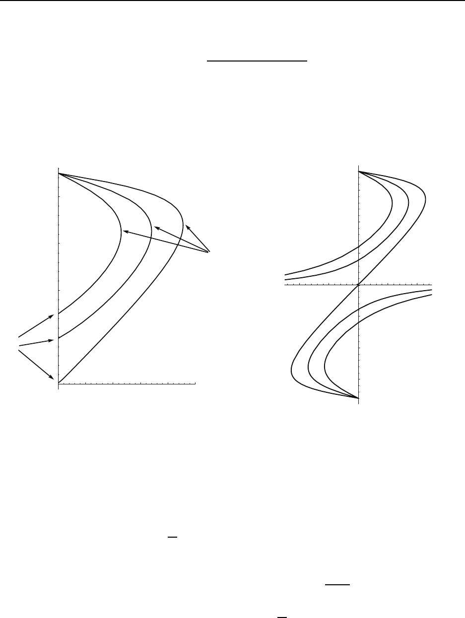
132 CHAPTER 5. STEADY SUPERSONIC TWO-DIMENSIONAL FLOW
With a little more algebra and trigonometry this reduces to
tan θ = 2cotβ
M
2
1
sin
2
β − 1
M
2
1
(γ + cos 2β) + 2
(5.53)
Given M
1
, γ and β, this equation can be solved to find θ the wedge angle. It can be inverted
to form an equation cubic in sin β to solve explicitly for β. Figure 5.3 gives a plot of oblique
shock angle β versus wedge angle θ.
β
θ
90
60
30
0
0 10 20 30 40 50
γ = 7/5
Μ
1
= 2
Μ
1
= 3
Μ
1
= ∞
maximum wedge
angle for attached
oblique shock
strong branch
(post-shock subsonic)
weak branch
(post shock supersonic, primarily)
-75
-50
-25
25
50
75
-40 -20
20
40
expanded view of β−θ plane
2nd law
violation
2nd Law
Violation
Μ
1
= 2
Μ
1
= 3
Μ
1
= ∞
β
θ
Figure 5.3: Shock angle β versus wedge ang le θ
Note t he following features:
• for a given θ < θ
max
, there exist two β’s
– lower β is weak solution
∗ lim
θ →0
β = arcsin
1
M
, a Mach wave
∗ relevant bra nch for most external flows, matches in far-field to acoustic wave,
can exist in internal flows
∗ total Mach number primarily supersonic, M
2
2
=
˜u
2
+˜v
2
c
2
2
> 1 for nearly all 0 <
θ < θ
max
∗ normal Mach number subsonic, M
2
2n
=
˜u
2
c
2
2
< 1
CC BY-NC-ND. 28 October 2019, J. M. Powers.
5.3. OBLIQUE SHOCK WAVES 133
– higher β is the strong solution
∗ lim
θ →0
β =
π
2
, a normal shock wave
∗ relevant branch for some internal flows
∗ total Mach number completely subsonic, M
2
2
=
˜u
2
+˜v
2
c
2
2
< 1 for all 0 < θ < θ
max
∗ normal Mach number subsonic, M
2
2n
=
˜u
2
c
2
2
< 1
• for θ > θ
max
, no solution exists; shock becomes detached
• Consider fixed θ, increasing freestream Mach number M
1
, see Figure 5.4
– 0 < M
1
< 1, subsonic incoming flow, no shocks continuous pressure variation
– 1 < M
1
< M
1a
, supersonic incoming flow, detached curved oblique shock
– M
1a
< M
1
< ∞, supersonic incoming flow, attached straight oblique shock
– as M
1
→ ∞, β → β
∞
• Consider fixed supersonic freestream Mach number M
1
, increasing θ, see Figure 5.5
– θ ∼ 0, Mach wave, negligible disturbance
– small θ, small β, small pressure, density rise
– medium θ, medium β, moderate pressure and density rise
– larg e θ, curved detached shock, large pressure and density rise
Example 5. 1
Oblique Shock Example
Given: Air flowing over a wedge, θ = 20
◦
, P
1
= 100 kP a, T
1
= 300 K, M
1
= 3.0
Find: Shock angle β and downstream pressur e and tempe rature P
2
, T
2
.
Assume: calorically perfect ideal gas
Analysis:
First some preliminaries:
c
1
=
p
γRT
1
=
s
(1.4)
287
J
kg K
(300 K) = 347.2
m
s
(5.54)
u
1
= M
1
c
1
= (3.0)
347.2
m
s
= 1, 041.6
m
s
(5.55)
ρ
1
=
P
1
RT
1
=
100, 000 P a
287
J
kg K
(300 K)
= 1.1614
kg
m
3
(5.56)
CC BY-NC-ND. 28 October 2019, J. M. Powers.

134 CHAPTER 5. STEADY SUPERSONIC TWO-DIMENSIONAL FLOW
M
1
< 1
subsonic, shockless flow
M
1
~ 1
slightly supersonic flow
shock approaching
wedge from infinity
continuous pressure
variation
1 < M
1
< M
1a
moderately supersonic flow
detached
oblique shock
M
1a
< M
1
<
∞
M
1
->
∞
attached
oblique shock
attached
oblique shock
at limiting wave
angle
β
min
Figure 5.4: Shock wave patterns as incoming Mach number varied
Now find the wave angle:
tan θ = 2cotβ
M
2
1
sin
2
β − 1
M
2
1
(γ + cos 2β) + 2
(5.57)
tan 20
◦
= 2cotβ
3.0
2
sin
2
β −1
3.0
2
(1.4 + cos 2β) + 2
(5.58)
(5.59)
Three solutions:
weak oblique shock; co mmon β = 3 7.76
◦
(5.60)
strong o blique shock; ra re β = 82.15
◦
(5.61)
second law violating “rarefa c tion” shock β = −9.91
◦
(5.62)
1. Weak Obliq ue Shock
˜u
1
= u
1
sin β =
1, 041.6
m
s
sin 37.76
◦
= 637.83
m
s
(5.63)
˜v
1
= u
1
cos β =
1, 041.6
m
s
cos 37.76
◦
= 823.47
m
s
(5.64)
M
1n
=
˜u
1
c
1
=
637.83
m
s
347.2
m
s
= 1.837 (5.65)
ρ
1
ρ
2
=
γ − 1
γ + 1
1 +
2
(γ − 1) M
2
1n
(5.66)
CC BY-NC-ND. 28 October 2019, J. M. Powers.

5.3. OBLIQUE SHOCK WAVES 135
M
1
M
1
M
1
M
1
Mach wave
small disturbance
attached shocks
moderate disturbances
detached shock
large disturbance
M
1
xed, supersonic, P
1
, ρ
1
xed
Figure 5.5: Shock wave patterns as wedge angle varied
1.1614
kg
m
3
ρ
2
=
1.4 −1
1.4 + 1
1 +
2
(1.4 −1 ) 1.837
2
= 0.413594 (5.67)
ρ
2
=
1.1614
kg
m
3
0.41359
= 2.8081
kg
m
3
(5.68)
ρ
2
˜u
2
= ρ
1
˜u
1
(5.69)
˜u
2
=
ρ
1
˜u
1
ρ
2
=
1.1614
kg
m
3
637.83
m
s
2.8081
kg
m
3
= 263.80
m
s
(5.70)
˜v
2
= ˜v
1
= 823.47
m
s
(5.71)
u
2
= ˜u
2
sin β + ˜v
2
cos β (5.72)
v
2
= −˜u
2
cos β + ˜v
2
sin β (5.73)
u
2
=
263.80
m
s
sin 37.76
◦
+
823.47
m
s
cos 37.76
◦
= 812.56
m
s
(5.74)
v
2
= −
263.80
m
s
cos 37.76
◦
+
823.47
m
s
sin 37.76
◦
= 295.70
m
s
(5.75)
check on wedge angle θ = arctan
v
2
u
2
(5.76)
= arctan
295.70
m
s
812.56
m
s
= 19.997
◦
(5.77)
P
2
= P
1
+ ρ
1
˜u
2
1
− ρ
2
˜u
2
2
(5.78)
P
2
= 100, 000 P a +
1.1614
kg
m
3
637.83
m
s
2
−
2.8081
kg
m
3
263.80
m
s
2
(5.79)
P
2
= 377, 072 P a (5.8 0)
T
2
=
P
2
ρ
2
R
=
377, 072 P a
2.8081
kg
m
3
287
J
kg K
= 467.88 K (5.81)
c
2
=
p
γRT
2
=
s
(1.4)
287
J
kg K
(467.88 K) = 43 3.58
m
s
(5.82)
CC BY-NC-ND. 28 October 2019, J. M. Powers.

136 CHAPTER 5. STEADY SUPERSONIC TWO-DIMENSIONAL FLOW
M
2n
=
˜u
2
c
2
=
263.8
m
s
433.58
m
s
= 0.608 (5.83)
M
2
=
p
u
2
2
+ v
2
2
c
2
=
q
812.56
m
s
2
+
295.7
m
s
2
433.58
m
s
= 1.994 (5.84)
s
2
− s
1
= c
p
ln
T
2
T
1
− R ln
P
2
P
1
(5.85)
=
1, 004.5
J
kg K
ln
467.88 K
300 K
−
287
J
kg K
ln
377, 072 P a
100, 000 P a
(5.86)
s
2
− s
1
= 65.50
J
kg K
(5.87)
2. Strong Oblique Shock
˜u
1
= u
1
sin β =
1, 041.6
m
s
sin 82.15
◦
= 1, 031.84
m
s
(5.88)
˜v
1
= u
1
cos β =
1, 041.6
m
s
cos 82.15
◦
= 142.26
m
s
(5.89)
M
1n
=
˜u
1
c
1
=
1, 031.84
m
s
347.2
m
s
= 2.972 (5.90)
ρ
1
ρ
2
=
γ − 1
γ + 1
1 +
2
(γ − 1) M
2
1n
(5.91)
1.1614
kg
m
3
ρ
2
=
1.4 −1
1.4 + 1
1 +
2
(1.4 − 1) 2.972
2
= 0.26102 (5.92)
ρ
2
=
1.1614
kg
m
3
0.26102
= 4.4495
kg
m
3
(5.93)
ρ
2
˜u
2
= ρ
1
˜u
1
(5.94)
˜u
2
=
ρ
1
˜u
1
ρ
2
=
1.1614
kg
m
3
1, 031.84
m
s
4.4495
kg
m
3
= 269.33
m
s
(5.95)
˜v
2
= ˜v
1
= 142.26
m
s
(5.96)
u
2
= ˜u
2
sin β + ˜v
2
cos β (5.97)
v
2
= −˜u
2
cos β + ˜v
2
sin β (5.98)
u
2
=
269.33
m
s
sin 82.15
◦
+
142.26
m
s
cos 82.15
◦
= 286.24
m
s
(5.99)
v
2
= −
269.33
m
s
cos 82.15
◦
+
142.26
m
s
sin 82.15
◦
= 104.14
m
s
(5.100)
check on wedge angle θ = arctan
v
2
u
2
(5.101)
= arctan
104.14
m
s
286.24
m
s
= 19.99
◦
(5.102)
P
2
= P
1
+ ρ
1
˜u
2
1
− ρ
2
˜u
2
2
(5.103)
P
2
= 100, 000 P a +
1.1614
kg
m
3
1, 031.84
m
s
2
−
4.4495
kg
m
3
269.33
m
s
2
(5.104)
P
2
= 1, 013, 775 P a (5.105)
CC BY-NC-ND. 28 October 2019, J. M. Powers.

5.3. OBLIQUE SHOCK WAVES 137
T
2
=
P
2
ρ
2
R
=
1, 013, 775 P a
4.4495
kg
m
3
287
J
kg K
= 793.86 K (5.106)
c
2
=
p
γRT
2
=
s
(1.4)
287
J
kg K
(793.86 K) = 56 4.78
m
s
(5.107)
M
2n
=
˜u
2
c
2
=
269.33
m
s
564.78
m
s
= 0.477 (5.108)
M
2
=
p
u
2
2
+ v
2
2
c
2
=
q
286.24
m
s
2
+
104.14
m
s
2
564.78
m
s
= 0.539 (5.109)
s
2
− s
1
= c
p
ln
T
2
T
1
− R ln
P
2
P
1
(5.110)
=
1, 004.5
J
kg K
ln
793.86 K
300 K
−
287
J
kg K
ln
1, 013, 775 P a
100, 000 P a
(5.111)
s
2
− s
1
= 312.86
J
kg K
(5.112)
3. “Rarefaction Shock”
˜u
1
= u
1
sin β =
1, 041.6
m
s
sin (−9.91
◦
) = −179.26
m
s
(5.113)
˜v
1
= u
1
cos β =
1, 041.6
m
s
cos (−9.91
◦
) = 1, 0 26.06
m
s
(5.114)
M
1n
=
˜u
1
c
1
=
−179.26
m
s
347.2
m
s
= −0.5163 (5.115)
ρ
1
ρ
2
=
γ − 1
γ + 1
1 +
2
(γ − 1) M
2
1n
(5.116)
1.1614
kg
m
3
ρ
2
=
1.4 −1
1.4 + 1
1 +
2
(1.4 −1 ) (−0.5163)
2
!
= 3.2928 (5.117)
ρ
2
=
1.1614
kg
m
3
3.2928
= 0.3527
kg
m
3
(5.118)
ρ
2
˜u
2
= ρ
1
˜u
1
(5.119)
˜u
2
=
ρ
1
˜u
1
ρ
2
=
1.1614
kg
m
3
−179.26
m
s
0.3527
kg
m
3
= −590.27
m
s
(5.120)
˜v
2
= ˜v
1
= 1, 026.06
m
s
(5.121)
u
2
= ˜u
2
sin β + ˜v
2
cos β (5.122)
v
2
= −˜u
2
cos β + ˜v
2
sin β (5.123)
u
2
=
−590.27
m
s
sin (−9.91
◦
) +
1, 026.06
m
s
cos (−9.91
◦
) = 1, 1 12.34
m
s
(5.124)
v
2
= −
−590.27
m
s
cos (−9.91
◦
) +
1, 026.06
m
s
sin (−9.91
◦
) = 404.88
m
s
(5.125)
check on wedge angle θ = arctan
v
2
u
2
(5.126)
= arctan
404.88
m
s
1, 112.34
m
s
= 20.00
◦
(5.127)
CC BY-NC-ND. 28 October 2019, J. M. Powers.

138 CHAPTER 5. STEADY SUPERSONIC TWO-DIMENSIONAL FLOW
P
2
= P
1
+ ρ
1
˜u
2
1
− ρ
2
˜u
2
2
(5.128)
P
2
= 100, 000 P a +
1.1614
kg
m
3
−179.26
m
s
2
−
0.3527
kg
m
3
−590.27
m
s
2
(5.129)
P
2
= 14, 433 P a (5.130)
T
2
=
P
2
ρ
2
R
=
14, 433 P a
0.3527
kg
m
3
287
J
kg K
= 142.59 K (5.131)
c
2
=
p
γRT
2
=
s
(1.4)
287
J
kg K
(142.59 K) = 239.36
m
s
(5.132)
M
2n
=
˜u
2
c
2
=
−590.27
m
s
239.36
m
s
= −2.47 (5.133)
M
2
=
p
u
2
2
+ v
2
2
c
2
=
q
1, 112.34
m
s
2
+
404.88
m
s
2
239.36
m
s
= 4.95 (5.134)
s
2
− s
1
= c
p
ln
T
2
T
1
− R ln
P
2
P
1
(5.135)
=
1, 004.5
J
kg K
ln
142.59 K
300 K
−
287
J
kg K
ln
14, 433 P a
100, 000 P a
(5.136)
s
2
− s
1
= −191.5
J
kg K
(5.137)
5.4 Small disturbance theory
By taking a Taylor series expansion of the relationship between β and θ abo ut θ = 0, for
fixed M
1
and γ it can be shown that
tan β =
1
p
M
2
1
− 1
+
γ + 1
4
M
4
1
(M
2
1
− 1)
2
θ θ << 1 (5.138)
Note t hat when θ = 0 t hat
tan β =
1
p
M
2
1
− 1
(5.139)
tan
2
β =
1
M
2
1
− 1
(5.140)
sin
2
β
cos
2
β
=
sin
2
β
1 −sin
2
β
=
1
M
2
1
− 1
(5.141)
sin
2
β
1 −sin
2
β
=
1
M
2
1
1 −
1
M
2
1
(5.142)
CC BY-NC-ND. 28 October 2019, J. M. Powers.

5.4. SMALL DISTURBANCE THEORY 139
sin β =
1
M
1
(5.143)
β = arcsin
1
M
1
(5.144)
After a good deal of algebra and t rigonometry, it can also be shown that the pressure
change, change in velocity magnitude, w, and change in entropy for flow over a thin wedge is
P
2
− P
1
P
1
=
γM
2
1
p
M
2
1
− 1
θ (5.145)
w
2
− w
1
w
1
= −
θ
p
M
2
1
− 1
(5.146)
s
2
− s
1
s
1
∼ θ
3
(5.147)
In terms o f changes,
∆P
P
1
=
γM
2
1
p
M
2
1
− 1
∆θ (5.148)
∆w
w
1
= −
∆θ
p
M
2
1
− 1
(5.149)
∆s
s
1
∼ ∆θ
3
(5.150)
Note t hat a small positive ∆θ gives rise to
• an increase in pressure
• a decrease in velocity mag nitude
• a very small change in entropy
Figure 5.6 shows the pattern of waves that one obtains when subjecting a flow to a series
of small turns and the pattern t hat evolves as the turning radius is shrunk.
• compression waves converge
• expansion waves diverge
• convergence of compression waves leads to region of rapid entropy rise–shock formation
• divergence of pressure waves leads to no shock formation in expansion
This has an analog in one-dimensional unsteady flow. Consider a piston with an initial
velocity of zero accelerating into a tube
CC BY-NC-ND. 28 October 2019, J. M. Powers.

140 CHAPTER 5. STEADY SUPERSONIC TWO-DIMENSIONAL FLOW
Isentropic Compression
Wave convergence;
Shock Formation;
Breakdown of Isentropic Assumption
Isentropic Expansion
Wave divergence;
No shock formation
Prandtl-Meyer
Expansion
Oblique
Shock
Figure 5.6: Wave pattern and streamlines for flows undergoing a series of small turns and
for sudden turns
• lead compression wave travels a t sound speed
• lead wave increases temperature (and sound speed) of disturbed flow
• each successive acoustic wave travels faster than lead wave
• eventually acoustic waves catch and form a shock
Consider a piston with zero initial velocity which decelerates
• lead expansion wave travels at sound speed
• lead wave decreases temperature (and sound speed) of disturbed flow
• each successive acoustic wave travels slow than lead wave
• no shock format ion
A schematic for these one- dimensional unsteady flows is shown in Figure 5.7
CC BY-NC-ND. 28 October 2019, J. M. Powers.

5.5. CENTERED PRANDTL-MEYER RAREFACTION 141
x
x
t
t
accelerating
piston
path
slow, acoustic
lead wave
shock
decelerating
piston
path
x
t
suddenly
accelerated
piston path
shock
locus
x
t
suddenly
decelerated
piston
path
Prandtl-Meyer
expansion fan
P
1
, ρ
1
P
1
, ρ
1
Figure 5.7: Schematic of compression and expansion waves for one-dimensional unsteady
piston-driven flow
5.5 Centered Prandtl-Meyer rarefactio n
If we let ∆θ → 0, the entropy changes become negligibly small relat ive to pressure and
velocity changes, and the flow is isent r opic. The relations can be replaced by differential
relations:
dP
P
=
γM
2
√
M
2
− 1
dθ (5.151)
dw
w
= −
dθ
√
M
2
− 1
(5.152)
ds
s
∼ 0 ( 5.153)
CC BY-NC-ND. 28 October 2019, J. M. Powers.

142 CHAPTER 5. STEADY SUPERSONIC TWO-DIMENSIONAL FLOW
Recall now that for adiabatic flow
T
o
T
= 1 +
γ − 1
2
M
2
(5.154)
γRT
o
γRT
= 1 +
γ − 1
2
M
2
(5.155)
c
2
o
c
2
= 1 +
γ − 1
2
M
2
(5.156)
c = c
o
1 +
γ − 1
2
M
2
−
1
2
(5.157)
dc = −
c
o
2
1 +
γ − 1
2
M
2
−
3
2
(γ − 1) MdM (5.158)
dc
c
= −
γ−1
2
MdM
1 +
γ−1
2
M
2
(5.159)
Also
w = cM (5.160)
dw = cdM + Mdc (5.161)
dw
w
=
dM
M
+
dc
c
(5.162)
dw
w
=
dM
M
−
γ−1
2
MdM
1 +
γ−1
2
M
2
(5.163)
dw
w
=
1
1 +
γ−1
2
M
2
dM
M
(5.164)
−
dθ
√
M
2
− 1
=
1
1 +
γ−1
2
M
2
dM
M
(5.165)
−dθ =
√
M
2
− 1
M
dM
1 +
γ−1
2
M
2
(5.166)
Now positive θ corresponds t o compression and negative θ corresponds to expansion.
Let’s define ν so positive ν gives and expansion.
ν ≡ − θ + θ
o
(5.167)
dν = −dθ (5.168)
Now integrate the expression
dν =
√
M
2
− 1
M
dM
1 +
γ−1
2
M
2
(5.169)
CC BY-NC-ND. 28 October 2019, J. M. Powers.

5.5. CENTERED PRANDTL-MEYER RAREFACTION 143
Let ν = 0 correspond to M = 1 . This effectively selects θ
o
ν(M) =
r
γ + 1
γ − 1
tan
−1
r
γ − 1
γ + 1
(M
2
− 1) −tan
−1
√
M
2
− 1 (5.170)
The function ν(M) is called the Prandtl-Meyer function. It is plot t ed in F igure 5 .8.
Many texts t abulate the Prandtl-Meyer function. For a known turning angle, one can find
the Mach number. As the flow is entirely isentropic, all other flow variables can be obtained
through the isentropic relations. Note:
• As M → ∞, ν →
π
2
q
γ+1
γ−1
− 1
, cor r esponds to vacuum conditions
• given ν, o ne can calculate M
• isentropic relations give P , ρ, T , etc.
• Prandtl-Meyer function tabulated in many texts
10 20 30 40
60
80
100
120
γ = 7/5
ν (ο)
M
ν
max
= 130.5
ο
Figure 5.8: Prandtl-Meyer function
Example 5. 2
Centered Expansion
Given: C alorically perfect, ideal air with P
1
= 100 kP a, T
1
= 300 K, u
1
= 500
m
s
, turned through
a 30
◦
expansion corner.
Find: Fluid properties after the expansion
Analysis:
CC BY-NC-ND. 28 October 2019, J. M. Powers.

144 CHAPTER 5. STEADY SUPERSONIC TWO-DIMENSIONAL FLOW
ρ
1
=
P
1
RT
1
=
100 kP a
0.287
J
kg K
(300 K)
= 1.1614
kg
m
3
(5.171)
c
1
=
p
γRT
1
=
s
1.4
287
J
kg K
(300 K) = 34 7.2
m
s
(5.172)
M
1
=
u
1
c
1
=
500
m
s
347.2
m
s
= 1.4401 (5.173)
T
o
= T
1
1 +
γ − 1
2
M
2
1
(5.174)
T
o
= 300 K
1 +
1
5
1.4401
2
= 424.43 K (5.175)
P
o
= P
1
1 +
γ − 1
2
M
2
1
γ
γ−1
(5.176)
P
o
= 100 kP a
1 +
1
5
1.4401
2
3.5
= 336.828 k P a (5.17 7)
Now calculate the Prandtl-Meyer function for the freestream:
ν(M
1
) =
r
γ + 1
γ − 1
tan
−1
r
γ − 1
γ + 1
(M
2
1
− 1) − tan
−1
q
M
2
1
− 1 (5.178)
ν(M
1
) =
r
1.4 + 1
1.4 −1
tan
−1
r
1.4 −1
1.4 + 1
(1.4401
2
− 1) − tan
−1
p
1.4401
2
− 1 (5.179)
ν(M
1
) = 0.177138 rad (5.180)
ν(M
1
) = 0.177138 rad
180
◦
π rad
= 10.1493
◦
(5.181)
The interpretation here is that a n initially sonic flow would have had to had turned 10.1493
◦
to achieve
a Mach numb er of M
1
= 1.4401.
Now add on the actual turning:
ν(M
2
) = ν(M
1
) + 30
◦
(5.182)
ν(M
2
) = 10.1493
◦
+ 30
◦
= 40.1493
◦
(5.183)
ν(M
2
) = 40.1493
◦
π rad
180
◦
= 0.700737 rad (5.184)
A tr ial and error solution gives the M
2
which corresponds to ν(M
2
) = 0.700737 r ad:
0.700737 rad =
r
1.4 + 1
1.4 −1
tan
−1
r
1.4 −1
1.4 + 1
(M
2
2
− 1) −tan
−1
q
M
2
2
− 1 (5.185)
M
2
= 2.54431 (5.186)
T
2
= T
o
1 +
γ − 1
2
M
2
2
−1
(5.187)
T
2
= 424.43 K
1 +
1
5
2.54331
2
−1
= 189.4 K (5.188)
CC BY-NC-ND. 28 October 2019, J. M. Powers.

5.6. WAVE INTERACTIONS AND REFLECTIONS 1 45
P
2
= P
o
1 +
γ − 1
2
M
2
2
−
γ
γ−1
(5.189)
P
2
= 336.828 kP a
1 +
1
5
2.54331
2
−3.5
= 18.43 kP a (5.190)
ρ
2
=
P
2
RT
2
=
18.43 kP a
0.287
J
kg K
(189.4 K)
= 0.3390
kg
m
3
(5.191)
c
2
=
p
γRT
2
=
s
1.4
287
J
kg K
(189.4 K) = 275.87
m
s
(5.192)
w
2
= M
2
c
2
= 2.54431
275.87
m
s
= 701.89
m
s
(5.193)
5.6 Wave interacti ons and reflections
Shocks and rarefactions can intersect and reflect in a va r iety of ways.
5.6.1 Oblique shock reflected from a wall
An oblique shock which reflects from a wall is represented in Figure 5.9.
β
1
β
2
Μ
1
Μ
2
Μ
3
P
1
P
2
P
3
interior streamline
pressure field
P
1
P
3
wall pressure
Figure 5.9: Reflection o f an oblique shock from a wall
Note:
CC BY-NC-ND. 28 October 2019, J. M. Powers.

146 CHAPTER 5. STEADY SUPERSONIC TWO-DIMENSIONAL FLOW
• analysis just that of two oblique shocks
• flow always turns to be parallel to wall
• angle of incidence not equal angle of reflection due to non-linear effects
• interior pressure profile has two steps
• wall pressure profile has single step
• P
2
> 2P
1
, t hat is the pressure is h i gher than that obtained in the acoustic limit
5.6.2 Oblique shock intersection
Two oblique shocks intersect as sketched in Figure 5.10
Μ
1
Μ
2
Μ
3
Μ
2
Figure 5.10: Interaction of two oblique shocks
Note:
• flow always turns to be parallel to wall
• when shocks intersect, flow turns again to be par allel to itself
5.6.3 Shock strengthening
A flow turned by a corner through an oblique shock can be strengthened by a second tur n
as sketched in Figure 5.11
Note: three new waves generated
CC BY-NC-ND. 28 October 2019, J. M. Powers.

5.7. SUPERSONIC FLOW OVER AIRFOILS 147
slipstream
rarefaction
Figure 5.11: Shock Strengthening Sketch
• strengthened shock
• slipstream in which pressures match, velocity directions match, but velocity magnitudes
differ
• weak rarefaction wave
5.6.4 Shock weakening
A flow turned by a corner throug h an o blique shock can be weakened by a second turn as
sketched in Figure 5 .12
Figure 5.12: Shock Weakening Sketch
5.7 Supersoni c flow over airfoils
The standard problem in flow over an airfoil is to determine the lift and the drag. While in
actual design it is the magnitude of the lift for ce F
L
, a nd drag force F
D
, that is most crucial,
CC BY-NC-ND. 28 October 2019, J. M. Powers.

148 CHAPTER 5. STEADY SUPERSONIC TWO-DIMENSIONAL FLOW
there exists dimensionless numbers the lift coefficient C
L
and the drag coefficient C
D
which
give good relative measures of airfoil performance.
C
L
≡
F
L
1
2
ρ
1
u
2
1
A
(5.194)
C
D
≡
F
D
1
2
ρ
1
u
2
1
A
(5.195)
Though this is the traditional formula, it is proba bly not the best for interpreting how the
forces vary when flight speed is varied. This is because when u
1
, flight speed is varied both
numerator and denominator change. To remedy this, we can instead scale by the ambient
sound speed to define a dimensionless lift force F ∗
L
and dimensionless drag force F ∗
D
:
F ∗
L
≡
F
L
ρ
1
c
2
1
A
(5.196)
F ∗
D
≡
F
D
ρ
1
c
2
1
A
(5.197)
5.7.1 Flat plate at angle of attack
The simplest problem is that of a flat plate at ang le of attack α
o
. A schematic is illustrated
in Figure 5.13. Note:
P
2
P
2
'
P
1
T
1
M
1
α
ο
far
field
Mach
wave
far
field
Mach
wave
leading edge
rarefaction
leading edge
shock
slipstream
Figure 5.13: Supersonic Flow over a F lat Plate
• flow over the top is turned through an isentropic rarefaction to P
2
CC BY-NC-ND. 28 October 2019, J. M. Powers.

5.7. SUPERSONIC FLOW OVER AIRFOILS 149
• flow over the bott om is turned t hrough an oblique shock to P
′
2
• Since P
′
2
> P
2
, t here is both lift and drag forces!
• both a shock and rarefaction are att ached to the trailing edge to turn the flow to the
horizontal
• the flow regions are separated by a slipstream in which pressure and velocity directions
match
• F
L
= (P
′
2
− P
2
) A cos α
o
, C
L
=
(
P
′
2
−P
2
)
cos α
o
1
2
ρ
1
u
2
1
• F
D
= (P
′
2
− P
2
) A sin α
o
, C
D
=
(
P
′
2
−P
2
)
sin α
o
1
2
ρ
1
u
2
1
• the drag here is known as wave drag or induced drag
• other components of drag, skin fric tion drag and thickness drag are zero due t o inviscid
limit and zero thickness limit
In the small disturbance limit
∆P
P
1
=
γM
2
1
p
M
2
1
− 1
∆θ (5.1 98)
P
′
2
= P
1
+
γP
1
M
2
1
p
M
2
1
− 1
α
o
(5.199)
P
2
= P
1
+
γP
1
M
2
1
p
M
2
1
− 1
(−α
o
) (5.200)
P
′
2
− P
2
=
2γP
1
M
2
1
p
M
2
1
− 1
α
o
(5.201)
P
′
2
− P
2
=
2γP
1
p
M
2
1
− 1
u
2
1
γP
1
ρ
1
α
o
(5.202)
P
′
2
− P
2
=
2
p
M
2
1
− 1
ρ
1
u
2
1
α
o
(5.203)
F
L
=
2
p
M
2
1
− 1
ρ
1
u
2
1
α
o
A cos α
o
(5.204)
F
L
=
2
p
M
2
1
− 1
ρ
1
u
2
1
α
o
A(1) (5.205)
C
L
=
4α
o
p
M
2
1
− 1
(5.206)
CC BY-NC-ND. 28 October 2019, J. M. Powers.

150 CHAPTER 5. STEADY SUPERSONIC TWO-DIMENSIONAL FLOW
F
D
=
2
p
M
2
1
− 1
ρ
1
u
2
1
α
o
A sin α
o
(5.207)
F
D
=
2
p
M
2
1
− 1
ρ
1
u
2
1
α
2
o
A (5.208)
C
D
=
4 α
2
o
p
M
2
1
− 1
(5.209)
F ∗
L
=
F
L
ρ
1
c
2
1
A
=
2 M
2
1
α
o
p
M
2
1
− 1
(5.210)
F ∗
D
=
F
D
ρ
1
c
2
1
A
=
2 M
2
1
α
2
o
p
M
2
1
− 1
(5.211)
High Mach number limit: F ∗
L
= 2M
1
α
o
(5.212)
High Mach number limit: F ∗
D
= 2M
1
α
2
o
(5.213)
Dimensionless lift and drag are plotted versus Mach number in Figure 5.14
Example 5. 3
Lift and Drag on an Inclined Flat Plate
Given: Flat plate, of chord length 2 m, depth 10 m inclined at 20
◦
to the horizontal in a freestream
of M
1
= 3, P
1
= 100 kP a, T
1
= 300 K.
Find: Lift and drag forces on the plate.
Analysis: First some preliminaries :
c
1
=
p
γRT
1
=
s
(1.4)
287
J
kg K
(300 K) = 347.2
m
s
(5.214)
u
1
= M
1
c
1
= (3.0)
347.2
m
s
= 1, 041.6
m
s
(5.215)
ρ
1
=
P
1
RT
1
=
100, 000 P a
287
J
kg K
(300 K)
= 1.1614
kg
m
3
(5.216)
P
o
= P
1
1 +
γ − 1
2
M
2
1
γ
γ−1
(5.217)
P
o
= 100 kP a
1 +
1
5
3
2
3.5
= 367.327 kP a (5.218)
In a previous example, we found the oblique shock state under identical conditio ns:
P
′
2
= 377, 072 P a (5.219)
Now consider the rarefaction.
CC BY-NC-ND. 28 October 2019, J. M. Powers.

5.7. SUPERSONIC FLOW OVER AIRFOILS 151
0
2
4
6 8 10
0.25
0.5
0.75
1
1.25
1.5
1.75
2
0
2
4
6 8 10
0.1
0.2
0.3
0.4
0.5
F* = F / ρ c A
M
1
1
1
L L
α = 5
ο
ο
F* = F / ρ c A
1 1 D D
2
2
Dimensionless Lift Force
Dimensionless Drag Force
α = 5
ο
ο
Flat Plate at Small Angle of Attack
Flat Plate at Small Angle of Attack
Invalid Region
Invalid Region
M
1
Figure 5.14: Dimensionless Lift and Dr ag versus Incoming Mach Number for Flat Plate at
Small Angle of Attack
ν(M
1
) =
r
γ + 1
γ − 1
tan
−1
r
γ − 1
γ + 1
(M
2
1
− 1) − tan
−1
q
M
2
1
− 1 (5.220 )
ν(M
1
) =
r
1.4 + 1
1.4 −1
tan
−1
r
1.4 −1
1.4 + 1
(3
2
− 1) −tan
−1
p
3
2
− 1 = 0.8691 rad = 49.7973
◦
(5.221)
ν(M
2
) = ν(M
1
) + 2 0
◦
(5.222)
ν(M
2
) = 49.7973
◦
+ 20
◦
= 69.7973
◦
(5.223)
69.7973
◦
= 1.218 rad =
r
1.4 + 1
1.4 −1
tan
−1
r
1.4 −1
1.4 + 1
(M
2
2
− 1) − tan
−1
q
M
2
2
− 1 (5.224 )
M
2
= 4.3209 (5.225)
P
2
= P
o
1 +
γ − 1
2
M
2
2
−
γ
γ−1
(5.226)
P
2
= 367.327 kP a
1 +
1
5
4.3209
2
−3.5
= 1.591 kP a (5.22 7)
CC BY-NC-ND. 28 October 2019, J. M. Powers.

152 CHAPTER 5. STEADY SUPERSONIC TWO-DIMENSIONAL FLOW
F
L
= (P
′
2
− P
2
) A cos α
o
(5.228)
F
L
= (377, 072 P a − 1, 591 P a) (10 m) (2 m ) cos 20
◦
(5.229)
F
L
= 7, 142, 073 N (5.230)
C
L
=
F
L
1
2
ρ
1
u
2
1
A
=
7, 142, 073 N
1
2
1.1614
kg
m
3
1, 041.6
m
s
2
(10 m) (2 m)
(5.231)
C
L
= 0.5668 (5.232)
F
D
= (P
′
2
− P
2
) A sin α
o
(5.233)
F
D
= (377, 072 P a − 1, 591 P a) (10 m) (2 m ) sin 20
◦
(5.234)
F
D
= 2, 320, 600 N (5.235)
C
D
=
F
D
1
2
ρ
1
u
2
1
A
=
2, 320, 600 N
1
2
1.1614
kg
m
3
1, 041.6
m
s
2
(10 m) (2 m)
(5.236)
C
D
= 0.1842 (5.237)
Compare with thin airfoil theory: C
L thin
=
4α
o
p
M
2
1
− 1
(5.238)
C
L thin
=
4 (20
◦
)
π ra d
180
◦
√
3
2
− 1
= 0.4936 (5.239)
C
D thin
=
4α
2
o
p
M
2
1
− 1
(5.240)
C
D thin
=
4
(20
◦
)
π rad
180
◦
2
√
3
2
− 1
= 0.1723 (5.241)
5.7.2 Diamond-shaped airfoil
The simplest supersonic airfo il with camber for analysis purposes is the diamond shaped
airfoil as sketched in Figure 5.15. The sketch shows the airf oil at zero angle of attack. The
upper half of the wedge is inclined at angle ǫ to the horizontal In this case there will be no
lift but there will be drag. Note the following features:
• sudden turn t hr ough lead oblique shock
• turn through isentropic Prandtl-Meyer rarefaction
• final turn through oblique shock attached to trailing edge
• far field limit: acoustic (Mach) waves
• Thin air foil limit C
L thin
=
4ǫ
√
M
2
1
−1
, same as f or flat plate!
• Thin air foil limit C
D thin
=
4ǫ
2
√
M
2
1
−1
, same as f or flat plate!
CC BY-NC-ND. 28 October 2019, J. M. Powers.

5.7. SUPERSONIC FLOW OVER AIRFOILS 153
2ε
P
1
T
1
M
1
P
2
P
3
P
4
far field
Mach waves
lead oblique
shock
trailing oblique
shock
Prandtl-Meyer
rarefaction
Figure 5.15: Supersonic Flow over a Diamond-Shaped Airfoil
5.7.3 General curved airfoil
A general airfoil with camber is sketched in Figure 5.16. The sketch shows the airfoil a t zero
angle of attack. In this case there will be no lift but there will be drag. Note the following
features:
• lead oblique shock
• lead shock weakened by series of no n-centered rarefaction waves
• shock at trailing edge, also weakened by non- centered r arefaction waves
• far field: acoustic (Mach) waves
5.7.4 Transonic transition
Transonic flow exists whenever there is a continuous transition from subsonic to supersonic
flow. One example of a transonic flow is sketched in Figure 5.17
1
which shows an accelerating
airfoil.
Note:
1
adopted from Bryson, A. E., “An Experimental Investigation of Transonic Flow Past Two-Dimensional
Wedge and Circular-Arc Sections Using a Mach-Zehnder Interfer ometer,” NACA Tech. Note 2560, 1951.
CC BY-NC-ND. 28 October 2019, J. M. Powers.

154 CHAPTER 5. STEADY SUPERSONIC TWO-DIMENSIONAL FLOW
Figure 5.16: Supersonic Flow over a Curved Airfoil
Μ
1
= 0.852
Μ
1
= 0.892
Μ
1
= 1.207 Μ
1
= 1.315 Μ
1
= 1.465
Shock
M < 1 M > 1 M < 1
Sonic Locus
Shock
Sonic Locus
M < 1
M > 1
M < 1
Shock
M < 1
M > 1
Sonic Locus
Shock
M < 1
M > 1
Shock
M < 1
M > 1
M > 1
M > 1
Figure 5.17: Tr ansition from Subsonic to Transonic to Supersonic Flow
• for hig h subsonic Mach number a bubble of supersonic flow appears
• smooth transition from subsonic to supersonic
• shock transition from supersonic to subsonic
• as Mach number increases, supersonic bubble expands
• for slightly supersonic Mach number, new shock approaches from far field
• as supersonic Mach number increases, shock from far field approaches leading edge and
supersonic bubble disappears
• challenging problems, not easily solved till 1960’s!
CC BY-NC-ND. 28 October 2019, J. M. Powers.

Chapter 6
Linear flow a na lysis
see Anderson, Ch apter 9
In this section we consider flows which are
• steady,
• two-dimensional,
• irrotational,
• isentropic,
• calorically perfect, and
• ideal.
The analysis is extensible to other cases.
6.1 Formulation
In lecture a detailed discussion is given in which the linearized velocity potential equation is
obtained:
1 − M
2
∞
∂
2
φ
∂x
2
+
∂
2
φ
∂y
2
= 0. (6.1)
6.2 Subson ic flow
Here we consider flows in which the Mach number is subsonic, but not negligibly small.
155

156 CHAPTER 6. LINEAR FLOW ANALYSIS
6.2.1 Prandtl-Glauret rule
A discussion is given where it is shown that the pressure coefficient on a supersonic airfoil
can be determined in terms of the pressure coefficient known from subsonic theory:
c
p
=
c
po
p
1 −M
2
∞
. (6.2)
6.2.2 Flow over wavy wall
The technique of separation o f variables is used to show the subsonic flow over a wavy wall
can be written in terms of the velocity potential as
φ(x, y) =
U
∞
h
p
1 − M
2
∞
sin
2πx
l
exp
−2π
p
1 −M
2
∞
y
l
!
. (6.3)
6.3 Supersoni c flow
6.3.1 D’Alembert’s solution
The D’Alembert solution for the wave equation is shown for supersonic flows:
φ(x, y) = f
x +
p
M
2
∞
− 1y
+ g
x −
p
M
2
∞
− 1y
. (6.4)
6.3.2 Flow over wavy wall
The solution for flow over a wavy wall is given in detail in lecture.
CC BY-NC-ND. 28 October 2019, J. M. Powers.

Chapter 7
Viscous flow
This chapter will focus on problems in which viscous stress plays an important role in deter-
mining the motion of the fluid. The topic in general is quite broad; to gain understanding
of the fundamental physics, we will restrict our a t t ention to the f ollowing limits:
• incompressible fluid
• isotropic Newtonian fluid with constant properties
• at most two-dimensional unsteady flow
The chapter will consider the governing equations and then solve a few representative
problems.
7.1 Gove r ning equations
This section considers the governing equations for the conditions specified for this chapter.
In dimensional non-conservative form, the governing equations are as follows:
∂u
∂x
+
∂v
∂y
= 0
ρ
∂u
∂t
+ ρu
∂u
∂x
+ ρv
∂u
∂y
= −
∂P
∂x
+ µ
∂
2
u
∂x
2
+
∂
2
u
∂y
2
ρ
∂v
∂t
+ ρu
∂v
∂x
+ ρv
∂v
∂y
= −
∂P
∂y
+ µ
∂
2
v
∂x
2
+
∂
2
v
∂y
2
ρc
p
∂T
∂t
+ u
∂T
∂x
+ v
∂T
∂y
=
∂P
∂t
+ u
∂P
∂x
+ v
∂P
∂y
+ k
∂
2
T
∂x
2
+
∂
2
T
∂y
2
+2µ
∂u
∂x
2
+
1
2
∂u
∂y
+
∂v
∂x
2
+
∂v
∂y
2
!
157

158 CHAPTER 7. VISCOUS FLOW
An argument could be made to eliminate the viscous dissipation term and the pressure
derivatives in the energy equation. The argument is subtle and based on the low Mach
number limit which corresponds to incompressibility.
7.2 Couette flow
Consider a channel flow driven by plate motion See Fig ure 7.1
x = 0
x
y
y = 0
y = h
U
P
0
T = T
T = T
0
0
P
0
Figure 7.1: Sketch for Couette flow
The mechanics of such a flow can b e described by stripping away many extraneous terms
from the governing equations.
Take
• fully developed velocity and temperature profiles:
∂u
∂x
≡ 0,
∂T
∂x
≡ 0
• steady flow
∂
∂t
≡ 0
• constant pressure field P (x, y, t) = P
o
• constant temperature channel walls T (x, 0, t) = T (x, h, t) = T
o
Since fully developed mass gives:
∂v
∂y
= 0 (7.1)
v(x, y) = f(x) (7.2)
and since in o r der to prevent ma ss flowing through the wall boundaries, v(x, 0) = v(x, h) = 0,
thus
CC BY-NC-ND. 28 October 2019, J. M. Powers.

7.2. COUETTE FLOW 159
v(x, y) = 0 (7.3)
Since
∂u
∂x
= 0,
∂u
∂t
= 0 and
∂T
∂x
= 0,
∂T
∂t
= 0, we have at most,
u = u(y) (7.4)
T = T (y) (7.5)
The y momentum equation has no information and x momentum and energy reduce to the
following:
0 = µ
d
2
u
dy
2
(7.6)
0 = k
d
2
T
dy
2
+ µ
du
dy
2
(7.7)
The x momentum equation is thus
d
2
u
dy
2
= 0 (7.8)
du
dy
= C
1
(7.9)
u(y) = C
1
y + C
2
(7.10)
Now applying u(0) = 0 and u(h) = U to fix C
1
and C
2
we get
u(y) = U
y
h
(7.11)
Shear stress:
τ
y x
= µ
∂u
∂y
(7.12)
τ
y x
= µ
U
h
(7.13)
The energy equation becomes
d
2
T
dy
2
= −
µ
k
du
dy
2
(7.14)
CC BY-NC-ND. 28 October 2019, J. M. Powers.

160 CHAPTER 7. VISCOUS FLOW
d
2
T
dy
2
= −
µ
k
U
2
h
2
(7.15)
dT
dy
= −
µ
k
U
2
h
2
y + C
1
(7.16)
T (y) = −
1
2
µ
k
U
2
h
2
y
2
+ C
1
y + C
2
(7.17)
Now T (0) = T
o
and T (h) = T
o
. This fixes the constants, so
T (y) =
1
2
µ
k
U
2
y
h
−
y
h
2
+ T
o
(7.18)
In dimensionless form this becomes
T −T
o
T
o
=
1
2
µc
p
k
U
2
c
p
T
o
y
h
−
y
h
2
(7.19)
T −T
o
T
o
=
P r Ec
2
y
h
−
y
h
2
(7.20)
Prandtl Number: P r ≡
µc
p
k
=
µ
ρ
k
ρc
p
=
ν
α
=
momentum diff usivity
thermal diffusivity
(7.21)
Eckert Number: Ec ≡
U
2
c
p
T
o
=
kinetic energy
thermal energy
(7.22)
Now
dT
dy
=
1
2
µ
k
U
2
h
2
(h − 2 y) (7.23)
q
y
= −k
dT
dy
=
1
2
µ
U
2
h
2
(2y − h) (7.24)
q
y
(0) = −
µU
2
2h
(7.25)
Note:
• at lower wall, heat flux into wall; heat generated in fluid conducted to wall
• wall heat flux magnitude independent of thermal conductivity
• higher plate velocity, higher wall heat flux
• higher viscosity, higher wall heat flux
• thinner gap, higher wall heat flux
CC BY-NC-ND. 28 October 2019, J. M. Powers.

7.3. SUDDENLY ACCELERATED FLAT PLATE 161
Also since T
max
occurs at y =
h
2
T
max
=
1
8
µ
k
U
2
+ T
o
(7.26)
Note:
• high viscosity, high maximum temperature
• high plate velocity, high maximum temperat ur e
• low thermal conductivity, high maximum temperature
Dimensionless wall heat flux given by the Nusselt number:
Nu ≡
q
y
(0)
k∆T
∆y
=
q
y
(0)∆y
k∆T
(7.27)
Nu =
µU
2
2h
h
2
k
1
8
µ
k
U
2
= 2 (7.28)
7.3 Sudden l y accelerate d flat plate
The problem of pulling a plate suddenly in a fluid which is initially at rest is o ften known
as Sto kes’ First Problem or Rayleigh’s problem.
7.3.1 Formulation
Consider a channel flow driven by a suddenly accelerated plate. See Figure 7.2 Initially,
t < 0
• fluid at rest
• plate at rest
For t ≥ 0
• plate pulled at constant velocity U
Assume:
• constant pressure P (x, y, t) = P
o
• fully developed flow
∂u
∂x
= 0,
∂T
∂x
= 0
CC BY-NC-ND. 28 October 2019, J. M. Powers.

162 CHAPTER 7. VISCOUS FLOW
U
ρ, µ,
u = u (y, t)
u(0,t) = U
u(∞, t) = 0
u (y, 0) = 0
x
y
δ ∼ (µ t / ρ)
1/2
P
0
T(∞, t) = T
0
T(y, t) = T
0
T(0, t) = T
0
Figure 7.2: Sketch fo r Stokes’ First Problem
Again from mass we deduce that v(x, y, t) = 0 . The x momentum equation reduces to
ρ
∂u
∂t
= µ
∂
2
u
∂y
2
(7.29)
The initial and boundary conditions are
u(y, 0) = 0 (7.30)
u(0, t) = U (7.31)
u(∞, t) = 0 (7.32)
7.3.2 Velocity profile
This problem is solved in detail in lecture. The solution for the velocity field is shown to be
u
U
o
= 1 −
2
√
π
Z
y /
√
νt
0
exp
−s
2
ds (7.33)
7.4 Starting transient for pl ane Couett e flow
The starting transient problem for plane Couette flow can be formulated as
∂u
∂t
= ν
∂
2
u
∂y
2
(7.34)
u(y, 0) = 0, u(0, t) = U
o
, u(h, t) = 0. (7.35)
In class a detailed solution is presented via the technique of separation of variables. The
solution is
CC BY-NC-ND. 28 October 2019, J. M. Powers.

7.5. BLASIUS BOUNDARY LAYER 163
u
U
o
= 1 −
y
h
−
2
π
∞
X
n=1
1
n
exp
−n
2
π
2
νt
h
2
sin
nπy
h
(7.36)
7.5 Blasius boundary layer
The problem of flow over a flat plate in the absence of pressure gradient is formulated and
solved using the classical approach of Blasius.
7.5.1 Formulation
After suitable scaling and definition of similarity variables, discussed in detail in class, the
following third order non-linear ordinary differential equation is obtained:
d
3
f
dη
3
+
1
2
f
d
2
f
dη
2
= 0, (7.37)
df
dη
η=0
= 0,
df
dη
η→∞
= 1, f|
η=0
= 0. (7.38)
This equation is solved numerically as a homework problem.
7.5.2 Wall shear stress
The solution is used to obtain t he classical formulae for skin friction coefficient:
C
f
=
0.664
√
Re
x
, (7.39)
and drag coefficient:
C
D
=
1.328
√
Re
L
. (7.40)
CC BY-NC-ND. 28 October 2019, J. M. Powers.


Chapter 8
Acoustics
This chapter outlines the brief introduction to acoustics given in class in somewhat more
detail.
8.1 Formulation
We reduce the Euler equations f or isentropic flow to the f ollowing equations where quantities
with a ha t are understood to be small perturbations about the ambient state, denoted with
a subscript o f ”o”.
∂ ˆρ
∂t
+ ρ
o
∇ ·
ˆ
v = 0 (8.1)
ρ
o
∂
ˆ
v
∂t
+ ∇·
ˆ
P = 0 (8.2)
ˆ
P = c
2
o
ˆρ. (8.3)
Introducing the velocity potential ∇φ =
ˆ
v and employing further manipulation allows the
equation to be written as the wave equation:
∂
2
φ
∂t
2
= c
2
o
∇
2
φ. (8.4)
The pressure, velocity, and density are then obtained fro m
ˆ
P = −ρ
o
∂φ
∂t
, (8.5)
ˆ
v = ∇φ, (8.6)
ˆρ = −ρ
o
c
2
o
∂φ
∂t
. (8.7)
165
166 CHAPTER 8. ACOUSTICS
8.2 Planar waves
The D’Alembert solution for planar waves is shown in class to be
φ = f (x + c
o
t) + g(x −c
o
t), (8.8)
ˆ
P = −ρ
o
c
o
f
′
(x + c
o
t) + ρ
o
c
o
g
′
(x − c
o
t), (8.9 )
ˆu = f
′
(x + c
o
t) + g
′
(x − c
o
t), (8.10)
(8.11)
8.3 Spherical waves
The D’Alembert solution for spherical waves is shown in class to be
φ =
1
r
f(r + c
o
t) +
1
r
g(r − c
o
t), (8.12)
ˆ
P = −
ρ
o
c
o
r
f
′
(r + c
o
t) +
ρ
o
c
o
r
g
′
(r −c
o
t), (8.13)
ˆu =
1
r
f
′
(r + c
o
t) +
1
r
g
′
(r − c
o
t), (8.14)
(8.15)
CC BY-NC-ND. 28 October 2019, J. M. Powers.
