Gas Dynamics Library User Guide

Easy5 2021.3

For Windows

and Linux

Main Index

Worldwide Web

www.mscsoftware.com

Support

http://www.mscsoftware.com/Contents/Services/Technical-Support/Contact-Technical-Support.aspx

Disclaimer

This documentation, as well as the software described in it, is furnished under license and may be used only in accordance with the

terms of such license.

MSC Software Corporation reserves the right to make changes in specifications and other information contained in this document

without prior notice.

The concepts, methods, and examples presented in this text are for illustrative and educational purposes only, and are not intended

to be exhaustive or to apply to any particular engineering problem or design. MSC Software Corporation assumes no liability or

responsibility to any person or company for direct or indirect damages resulting from the use of any information contained herein.

This notice shall be marked on any reproduction of this documentation, in whole or in part. Any reproduction or distribution of this

document, in whole or in part, without the prior written consent of MSC Software Corporation is prohibited.

This software may contain certain third-party software that is protected by copyright and licensed from MSC Software suppliers.

Additional terms and conditions and/or notices may apply for certain third party software. Such additional third party software terms

and conditions and/or notices may be set forth in documentation and/or at

http://www.mscsoftware.com/thirdpartysoftware (or successor

website designated by MSC from time to time). Portions of this software are owned by Siemens Product Lifecycle Management, Inc.

The MSC Software logo, MSC, MSC Adams, MD Adams, Adams and Easy5 are trademarks or registered trademarks of MSC Software

Corporation and/or its subsidiaries in the United States and other countries. Hexagon and the Hexagon logo are trademarks or

registered trademarks of Hexagon AB and/or its subsidiaries. NASTRAN is a registered trademark of NASA. FLEXlm and FlexNet

Publisher are trademarks or registered trademarks of Flexera Software. Parasolid is a registered trademark of Siemens Product

Lifecycle Management, Inc. All other trademarks are the property of their respective owners.

Use, duplicate, or disclosure by the U.S. Government is subjected to restrictions as set forth in FAR 12.212 (Commercial Computer

Software) and DFARS 227.7202 (Commercial Computer Software and Commercial Computer Software Documentation), as

applicable.

September 14, 2021

Corporate Europe, Middle East, Africa

MSC Software Corporation MSC Software GmbH

5161 California Ave, Suite 200 Am Moosfeld 13

University Research Park 81829 Munich, Germany

Irvine, CA 92617 Telephone: (49) 89 431 98 70

Telephone: (714) 540-8900 Email: [email protected]

Email: americas.contact@mscsoftware.com

Japan Asia-Pacific

MSC Software Japan Ltd. MSC Software (S) Pte. Ltd.

KANDA SQUARE 16F 100 Beach Road

2-2-1 Kanda Nishikicho, Chiyoda-ku #16-05 Shaw Tower

Tokyo 101-0054, Japan Singapore 189702

Telephone: (81)(3) 6275 0870 Telephone: 65-6272-0082

Email: MSCJ.Mark[email protected] Email: AP[email protected]

Main Index

Documentation Feedback

At MSC Software, we strive to produce the highest quality documentation and welcome your feedback.

If you have comments or suggestions about our documentation, write to us at:

documentation-

[email protected]

Please include the following information with your feedback:

 Document name

 Release/Version number

 Chapter/Section name

 Topic title (for Online Help)

 Brief description of the content (for example, incomplete/incorrect information, grammatical

errors, information that requires clarification or more details and so on).

 Your suggestions for correcting/improving documentation

You may also provide your feedback about MSC Software documentation by taking a short 5-minute

survey at:

http://msc-documentation.questionpro.com.

Note: The above mentioned e-mail address is only for providing documentation specific

feedback. If you have any technical problems, issues, or queries, please contact

Technical

Support

Main Index

Contents

Gas Dynamics Library User Guide

Contents

1 Overview

Introduction . . . . . . . . . . . . . . . . . . . . . . . . . . . . . . . . . . . . . . . . . . . . . . . . . . . . . . . . . . . . . . . . . . . . . . . . . 2

Key Features. . . . . . . . . . . . . . . . . . . . . . . . . . . . . . . . . . . . . . . . . . . . . . . . . . . . . . . . . . . . . . . . . . . . . . . . . 2

Formulation and Terminology . . . . . . . . . . . . . . . . . . . . . . . . . . . . . . . . . . . . . . . . . . . . . . . . . . . . . . . . . . . 3

Network Considerations. . . . . . . . . . . . . . . . . . . . . . . . . . . . . . . . . . . . . . . . . . . . . . . . . . . . . . . . . . . . . . . . 3

Flowstream Identification—Ports . . . . . . . . . . . . . . . . . . . . . . . . . . . . . . . . . . . . . . . . . . . . . . . . . . . . . . . 4

Species Identification . . . . . . . . . . . . . . . . . . . . . . . . . . . . . . . . . . . . . . . . . . . . . . . . . . . . . . . . . . . . . . . . 6

Global Configurations . . . . . . . . . . . . . . . . . . . . . . . . . . . . . . . . . . . . . . . . . . . . . . . . . . . . . . . . . . . . . . . . 6

Component Configurations . . . . . . . . . . . . . . . . . . . . . . . . . . . . . . . . . . . . . . . . . . . . . . . . . . . . . . . . . . . . 10

Component Types. . . . . . . . . . . . . . . . . . . . . . . . . . . . . . . . . . . . . . . . . . . . . . . . . . . . . . . . . . . . . . . . . . . . . 13

Actuators . . . . . . . . . . . . . . . . . . . . . . . . . . . . . . . . . . . . . . . . . . . . . . . . . . . . . . . . . . . . . . . . . . . . . . . . . 13

One-Dimensional Body Dynamics. . . . . . . . . . . . . . . . . . . . . . . . . . . . . . . . . . . . . . . . . . . . . . . . . . . . . . . 13

Boundary Conditions. . . . . . . . . . . . . . . . . . . . . . . . . . . . . . . . . . . . . . . . . . . . . . . . . . . . . . . . . . . . . . . . . 13

Forces and body dynamics . . . . . . . . . . . . . . . . . . . . . . . . . . . . . . . . . . . . . . . . . . . . . . . . . . . . . . . . . . . . 13

Compressor, Fan & Turbine . . . . . . . . . . . . . . . . . . . . . . . . . . . . . . . . . . . . . . . . . . . . . . . . . . . . . . . . . . . 14

Directional Control Valves. . . . . . . . . . . . . . . . . . . . . . . . . . . . . . . . . . . . . . . . . . . . . . . . . . . . . . . . . . . . . 14

Heat Exchangers . . . . . . . . . . . . . . . . . . . . . . . . . . . . . . . . . . . . . . . . . . . . . . . . . . . . . . . . . . . . . . . . . . . 14

Minor Losses . . . . . . . . . . . . . . . . . . . . . . . . . . . . . . . . . . . . . . . . . . . . . . . . . . . . . . . . . . . . . . . . . . . . . . 14

Miscellaneous . . . . . . . . . . . . . . . . . . . . . . . . . . . . . . . . . . . . . . . . . . . . . . . . . . . . . . . . . . . . . . . . . . . . . 15

Nodes and volumes . . . . . . . . . . . . . . . . . . . . . . . . . . . . . . . . . . . . . . . . . . . . . . . . . . . . . . . . . . . . . . . . . 15

Orifice and Nozzle . . . . . . . . . . . . . . . . . . . . . . . . . . . . . . . . . . . . . . . . . . . . . . . . . . . . . . . . . . . . . . . . . . 15

Pipes, lines and tubes. . . . . . . . . . . . . . . . . . . . . . . . . . . . . . . . . . . . . . . . . . . . . . . . . . . . . . . . . . . . . . . . 15

Sensors . . . . . . . . . . . . . . . . . . . . . . . . . . . . . . . . . . . . . . . . . . . . . . . . . . . . . . . . . . . . . . . . . . . . . . . . . . 16

Thermal Analysis . . . . . . . . . . . . . . . . . . . . . . . . . . . . . . . . . . . . . . . . . . . . . . . . . . . . . . . . . . . . . . . . . . . 16

Valves (each configurable as Resistive or Storage/Resistive). . . . . . . . . . . . . . . . . . . . . . . . . . . . . . . . . . . 16

Equations of State in the Gas Dynamics Library. . . . . . . . . . . . . . . . . . . . . . . . . . . . . . . . . . . . . . . . . . . . . 16

Guidelines for Building and Analyzing GD Models . . . . . . . . . . . . . . . . . . . . . . . . . . . . . . . . . . . . . . . . . . . 17

Connecting Components. . . . . . . . . . . . . . . . . . . . . . . . . . . . . . . . . . . . . . . . . . . . . . . . . . . . . . . . . . . . . . 17

System Size . . . . . . . . . . . . . . . . . . . . . . . . . . . . . . . . . . . . . . . . . . . . . . . . . . . . . . . . . . . . . . . . . . . . . . . 17

Data Entry . . . . . . . . . . . . . . . . . . . . . . . . . . . . . . . . . . . . . . . . . . . . . . . . . . . . . . . . . . . . . . . . . . . . . . . . 17

Error Controls . . . . . . . . . . . . . . . . . . . . . . . . . . . . . . . . . . . . . . . . . . . . . . . . . . . . . . . . . . . . . . . . . . . . . . 18

Model Operating Points . . . . . . . . . . . . . . . . . . . . . . . . . . . . . . . . . . . . . . . . . . . . . . . . . . . . . . . . . . . . . . 18

Main Index

Gas Dynamics Library User Guide

Steady-State Analysis . . . . . . . . . . . . . . . . . . . . . . . . . . . . . . . . . . . . . . . . . . . . . . . . . . . . . . . . . . . . . . . 19

References. . . . . . . . . . . . . . . . . . . . . . . . . . . . . . . . . . . . . . . . . . . . . . . . . . . . . . . . . . . . . . . . . . . . . . . . 20

2 Tutorial

Introduction . . . . . . . . . . . . . . . . . . . . . . . . . . . . . . . . . . . . . . . . . . . . . . . . . . . . . . . . . . . . . . . . . . . . . . . . . 22

The Conceptual Model . . . . . . . . . . . . . . . . . . . . . . . . . . . . . . . . . . . . . . . . . . . . . . . . . . . . . . . . . . . . . . . . . 22

Creating the Easy5 Block Diagram . . . . . . . . . . . . . . . . . . . . . . . . . . . . . . . . . . . . . . . . . . . . . . . . . . . . . . . 22

Adding Components . . . . . . . . . . . . . . . . . . . . . . . . . . . . . . . . . . . . . . . . . . . . . . . . . . . . . . . . . . . . . . . . . 23

Making Connections: Ports and Their Significance . . . . . . . . . . . . . . . . . . . . . . . . . . . . . . . . . . . . . . . . . . 24

Entering Data into the Model . . . . . . . . . . . . . . . . . . . . . . . . . . . . . . . . . . . . . . . . . . . . . . . . . . . . . . . . . . 28

Determining an Initial Operating Point . . . . . . . . . . . . . . . . . . . . . . . . . . . . . . . . . . . . . . . . . . . . . . . . . . . . 32

Simulating the System. . . . . . . . . . . . . . . . . . . . . . . . . . . . . . . . . . . . . . . . . . . . . . . . . . . . . . . . . . . . . . . . . 35

Using Easy5 to Analyze a More Complex System. . . . . . . . . . . . . . . . . . . . . . . . . . . . . . . . . . . . . . . . . . . . 39

3 Frequently Asked Questions

Frequently Asked Questions . . . . . . . . . . . . . . . . . . . . . . . . . . . . . . . . . . . . . . . . . . . . . . . . . . . . . . . . . . . . 46

4 Nodes and Volumes

Introduction . . . . . . . . . . . . . . . . . . . . . . . . . . . . . . . . . . . . . . . . . . . . . . . . . . . . . . . . . . . . . . . . . . . . . . . . . 50

Formulation and Terminology . . . . . . . . . . . . . . . . . . . . . . . . . . . . . . . . . . . . . . . . . . . . . . . . . . . . . . . . . . . 50

Fundamental Equations . . . . . . . . . . . . . . . . . . . . . . . . . . . . . . . . . . . . . . . . . . . . . . . . . . . . . . . . . . . . . . . . 50

Equation of State . . . . . . . . . . . . . . . . . . . . . . . . . . . . . . . . . . . . . . . . . . . . . . . . . . . . . . . . . . . . . . . . . . . 50

Equations of Continuity- Non-condensible gas species . . . . . . . . . . . . . . . . . . . . . . . . . . . . . . . . . . . . . . . 50

Equations of Continuity- Condensible gas species . . . . . . . . . . . . . . . . . . . . . . . . . . . . . . . . . . . . . . . . . . 51

Condensation Rate . . . . . . . . . . . . . . . . . . . . . . . . . . . . . . . . . . . . . . . . . . . . . . . . . . . . . . . . . . . . . . . . . . 51

Equation of Energy . . . . . . . . . . . . . . . . . . . . . . . . . . . . . . . . . . . . . . . . . . . . . . . . . . . . . . . . . . . . . . . . . . 52

Switch State Rate Calculation . . . . . . . . . . . . . . . . . . . . . . . . . . . . . . . . . . . . . . . . . . . . . . . . . . . . . . . . . . . 53

Guidelines for Component Selection. . . . . . . . . . . . . . . . . . . . . . . . . . . . . . . . . . . . . . . . . . . . . . . . . . . . . . 53

References . . . . . . . . . . . . . . . . . . . . . . . . . . . . . . . . . . . . . . . . . . . . . . . . . . . . . . . . . . . . . . . . . . . . . . . . . . 54

5 Orifices and Valves

Introduction . . . . . . . . . . . . . . . . . . . . . . . . . . . . . . . . . . . . . . . . . . . . . . . . . . . . . . . . . . . . . . . . . . . . . . . . . 56

Fundamental Equations . . . . . . . . . . . . . . . . . . . . . . . . . . . . . . . . . . . . . . . . . . . . . . . . . . . . . . . . . . . . . . . . 56

Orifice flow regimes. . . . . . . . . . . . . . . . . . . . . . . . . . . . . . . . . . . . . . . . . . . . . . . . . . . . . . . . . . . . . . . . . . . 56

Solution of the orifice equations . . . . . . . . . . . . . . . . . . . . . . . . . . . . . . . . . . . . . . . . . . . . . . . . . . . . . . . . . 57

Main Index

vii

Contents

Switch State Rate Calculation . . . . . . . . . . . . . . . . . . . . . . . . . . . . . . . . . . . . . . . . . . . . . . . . . . . . . . . . . . . 58

Valve/Duct Area Models (Components VD and VI) . . . . . . . . . . . . . . . . . . . . . . . . . . . . . . . . . . . . . . . . . . . 59

Poppet Valve Area (Component PA). . . . . . . . . . . . . . . . . . . . . . . . . . . . . . . . . . . . . . . . . . . . . . . . . . . . . . . 63

Component Selection- Orifices . . . . . . . . . . . . . . . . . . . . . . . . . . . . . . . . . . . . . . . . . . . . . . . . . . . . . . . . . . 63

References . . . . . . . . . . . . . . . . . . . . . . . . . . . . . . . . . . . . . . . . . . . . . . . . . . . . . . . . . . . . . . . . . . . . . . . . . . 63

6 Pipes and Flow Resistances

Introduction . . . . . . . . . . . . . . . . . . . . . . . . . . . . . . . . . . . . . . . . . . . . . . . . . . . . . . . . . . . . . . . . . . . . . . . . . 66

Discretization of PC and PX . . . . . . . . . . . . . . . . . . . . . . . . . . . . . . . . . . . . . . . . . . . . . . . . . . . . . . . . . . . . . 66

Fundamental Equations- Lumped Parameter, Transient Momentum . . . . . . . . . . . . . . . . . . . . . . . . . . . . 67

Equations of Continuity . . . . . . . . . . . . . . . . . . . . . . . . . . . . . . . . . . . . . . . . . . . . . . . . . . . . . . . . . . . . . . . 67

Condensation Rate . . . . . . . . . . . . . . . . . . . . . . . . . . . . . . . . . . . . . . . . . . . . . . . . . . . . . . . . . . . . . . . . . . 67

Equation of Energy . . . . . . . . . . . . . . . . . . . . . . . . . . . . . . . . . . . . . . . . . . . . . . . . . . . . . . . . . . . . . . . . . . 68

Heat Transfer Calculation . . . . . . . . . . . . . . . . . . . . . . . . . . . . . . . . . . . . . . . . . . . . . . . . . . . . . . . . . . . . . 68

Equation of Momentum. . . . . . . . . . . . . . . . . . . . . . . . . . . . . . . . . . . . . . . . . . . . . . . . . . . . . . . . . . . . . . . 69

Switch State Rate Calculation . . . . . . . . . . . . . . . . . . . . . . . . . . . . . . . . . . . . . . . . . . . . . . . . . . . . . . . . . . 72

Method of Characteristics . . . . . . . . . . . . . . . . . . . . . . . . . . . . . . . . . . . . . . . . . . . . . . . . . . . . . . . . . . . . . . 73

Flow Resistances and the Minor Loss group . . . . . . . . . . . . . . . . . . . . . . . . . . . . . . . . . . . . . . . . . . . . . . . 74

Guidelines for Component Selection and Use . . . . . . . . . . . . . . . . . . . . . . . . . . . . . . . . . . . . . . . . . . . . . . . 74

References . . . . . . . . . . . . . . . . . . . . . . . . . . . . . . . . . . . . . . . . . . . . . . . . . . . . . . . . . . . . . . . . . . . . . . . . . . 75

7 Heat Exchangers

Introduction . . . . . . . . . . . . . . . . . . . . . . . . . . . . . . . . . . . . . . . . . . . . . . . . . . . . . . . . . . . . . . . . . . . . . . . . . 78

Heat Exchangers Based on Effectiveness Maps . . . . . . . . . . . . . . . . . . . . . . . . . . . . . . . . . . . . . . . . . . . . . 78

Gas/Gas Heat Exchanger. . . . . . . . . . . . . . . . . . . . . . . . . . . . . . . . . . . . . . . . . . . . . . . . . . . . . . . . . . . . . . 78

Gas/Liquid Heat Exchanger . . . . . . . . . . . . . . . . . . . . . . . . . . . . . . . . . . . . . . . . . . . . . . . . . . . . . . . . . . . . 80

Limitations of Transient Analysis Using Effectiveness Models . . . . . . . . . . . . . . . . . . . . . . . . . . . . . . . . . . 80

Heat Exchangers- Single Pressure State, Discretized Temperature Array . . . . . . . . . . . . . . . . . . . . . . . . 81

Equations of Continuity . . . . . . . . . . . . . . . . . . . . . . . . . . . . . . . . . . . . . . . . . . . . . . . . . . . . . . . . . . . . . . . 81

Condensation Rate . . . . . . . . . . . . . . . . . . . . . . . . . . . . . . . . . . . . . . . . . . . . . . . . . . . . . . . . . . . . . . . . . . 82

Equation of Energy . . . . . . . . . . . . . . . . . . . . . . . . . . . . . . . . . . . . . . . . . . . . . . . . . . . . . . . . . . . . . . . . . . 82

Transient Response . . . . . . . . . . . . . . . . . . . . . . . . . . . . . . . . . . . . . . . . . . . . . . . . . . . . . . . . . . . . . . . . . 82

Heat Exchangers- Discretized Pressure and Temperature Vector . . . . . . . . . . . . . . . . . . . . . . . . . . . . . . . 82

Heat Transfer Coefficient Calculation (Components HE, HF, HS and HT) . . . . . . . . . . . . . . . . . . . . . . . . . . 83

Heat Exchanger Flow Calculation . . . . . . . . . . . . . . . . . . . . . . . . . . . . . . . . . . . . . . . . . . . . . . . . . . . . . . . . 83

Tabular Correlation . . . . . . . . . . . . . . . . . . . . . . . . . . . . . . . . . . . . . . . . . . . . . . . . . . . . . . . . . . . . . . . . . . 83

Analytical Correlation . . . . . . . . . . . . . . . . . . . . . . . . . . . . . . . . . . . . . . . . . . . . . . . . . . . . . . . . . . . . . . . . 83

Main Index

Gas Dynamics Library User Guide

viii

Steady-momentum pipe model (equivalent pipe) . . . . . . . . . . . . . . . . . . . . . . . . . . . . . . . . . . . . . . . . . . . 83

Zero-resistance flow-through. . . . . . . . . . . . . . . . . . . . . . . . . . . . . . . . . . . . . . . . . . . . . . . . . . . . . . . . . . 83

Transient-momentum pipe model (equivalent pipe) . . . . . . . . . . . . . . . . . . . . . . . . . . . . . . . . . . . . . . . . . 84

Switch State Rate Calculation . . . . . . . . . . . . . . . . . . . . . . . . . . . . . . . . . . . . . . . . . . . . . . . . . . . . . . . . . . . 84

Guidelines for Component Selection and Use. . . . . . . . . . . . . . . . . . . . . . . . . . . . . . . . . . . . . . . . . . . . . . . 85

Bibliography . . . . . . . . . . . . . . . . . . . . . . . . . . . . . . . . . . . . . . . . . . . . . . . . . . . . . . . . . . . . . . . . . . . . . . . . . 85

8 Chemical Reactors

Introduction . . . . . . . . . . . . . . . . . . . . . . . . . . . . . . . . . . . . . . . . . . . . . . . . . . . . . . . . . . . . . . . . . . . . . . . . . 88

Mathematical Model . . . . . . . . . . . . . . . . . . . . . . . . . . . . . . . . . . . . . . . . . . . . . . . . . . . . . . . . . . . . . . . . . . 88

Stoichiometric Coefficients. . . . . . . . . . . . . . . . . . . . . . . . . . . . . . . . . . . . . . . . . . . . . . . . . . . . . . . . . . . . 88

Extent of Reaction . . . . . . . . . . . . . . . . . . . . . . . . . . . . . . . . . . . . . . . . . . . . . . . . . . . . . . . . . . . . . . . . . . 90

Equilibrium Extent of Reaction . . . . . . . . . . . . . . . . . . . . . . . . . . . . . . . . . . . . . . . . . . . . . . . . . . . . . . . . . 90

Adiabatic Reaction Temperature. . . . . . . . . . . . . . . . . . . . . . . . . . . . . . . . . . . . . . . . . . . . . . . . . . . . . . . . 91

Non-adiabatic Reactor Modeling . . . . . . . . . . . . . . . . . . . . . . . . . . . . . . . . . . . . . . . . . . . . . . . . . . . . . . . 92

Guidelines for Component Selection and Use. . . . . . . . . . . . . . . . . . . . . . . . . . . . . . . . . . . . . . . . . . . . . . . 92

Bibliography . . . . . . . . . . . . . . . . . . . . . . . . . . . . . . . . . . . . . . . . . . . . . . . . . . . . . . . . . . . . . . . . . . . . . . . . . 92

9 Compressors, Fans, & Turbines

Introduction . . . . . . . . . . . . . . . . . . . . . . . . . . . . . . . . . . . . . . . . . . . . . . . . . . . . . . . . . . . . . . . . . . . . . . . . . 94

Compressors . . . . . . . . . . . . . . . . . . . . . . . . . . . . . . . . . . . . . . . . . . . . . . . . . . . . . . . . . . . . . . . . . . . . . . . . 94

Compressor Based upon Corrected Flow Map (CN). . . . . . . . . . . . . . . . . . . . . . . . . . . . . . . . . . . . . . . . . . 94

Compressor Based upon Map of Polytropic Efficiency and Polytropic Head (CP) . . . . . . . . . . . . . . . . . . . . 96

Fan . . . . . . . . . . . . . . . . . . . . . . . . . . . . . . . . . . . . . . . . . . . . . . . . . . . . . . . . . . . . . . . . . . . . . . . . . . . . . . . . 98

Turbine . . . . . . . . . . . . . . . . . . . . . . . . . . . . . . . . . . . . . . . . . . . . . . . . . . . . . . . . . . . . . . . . . . . . . . . . . . . . . 98

A Gas Properties

Accessing Gas Properties from FORTRAN or Macro Code . . . . . . . . . . . . . . . . . . . . . . . . . . . . . . . . . . . . . 102

Molar Volume. . . . . . . . . . . . . . . . . . . . . . . . . . . . . . . . . . . . . . . . . . . . . . . . . . . . . . . . . . . . . . . . . . . . . . 102

Enthalpy () . . . . . . . . . . . . . . . . . . . . . . . . . . . . . . . . . . . . . . . . . . . . . . . . . . . . . . . . . . . . . . . . . . . . . . . . 102

Entropy () . . . . . . . . . . . . . . . . . . . . . . . . . . . . . . . . . . . . . . . . . . . . . . . . . . . . . . . . . . . . . . . . . . . . . . . . . 103

Ideal Gas Heat Capacity . . . . . . . . . . . . . . . . . . . . . . . . . . . . . . . . . . . . . . . . . . . . . . . . . . . . . . . . . . . . . . 104

Non-Ideal Gas Heat Capacity . . . . . . . . . . . . . . . . . . . . . . . . . . . . . . . . . . . . . . . . . . . . . . . . . . . . . . . . . . 104

Viscosity . . . . . . . . . . . . . . . . . . . . . . . . . . . . . . . . . . . . . . . . . . . . . . . . . . . . . . . . . . . . . . . . . . . . . . . . . 104

ThermalConductivity . . . . . . . . . . . . . . . . . . . . . . . . . . . . . . . . . . . . . . . . . . . . . . . . . . . . . . . . . . . . . . . . 105

Partial Derivatives of Molar Volume . . . . . . . . . . . . . . . . . . . . . . . . . . . . . . . . . . . . . . . . . . . . . . . . . . . . . 105

Gas Density . . . . . . . . . . . . . . . . . . . . . . . . . . . . . . . . . . . . . . . . . . . . . . . . . . . . . . . . . . . . . . . . . . . . . . . 106

Species Densities. . . . . . . . . . . . . . . . . . . . . . . . . . . . . . . . . . . . . . . . . . . . . . . . . . . . . . . . . . . . . . . . . . . 107

Main Index

Contents

Partial Derivatives of Density . . . . . . . . . . . . . . . . . . . . . . . . . . . . . . . . . . . . . . . . . . . . . . . . . . . . . . . . . . 108

Densities and Partial Derivatives of Species Densities. . . . . . . . . . . . . . . . . . . . . . . . . . . . . . . . . . . . . . . . 108

Temperature Conversion. . . . . . . . . . . . . . . . . . . . . . . . . . . . . . . . . . . . . . . . . . . . . . . . . . . . . . . . . . . . . . 109

Total Pressure and Mole Fraction . . . . . . . . . . . . . . . . . . . . . . . . . . . . . . . . . . . . . . . . . . . . . . . . . . . . . . . 109

Critical Properties for Non-Ideal Gas Laws . . . . . . . . . . . . . . . . . . . . . . . . . . . . . . . . . . . . . . . . . . . . . . . . 110

User-Defined Gases . . . . . . . . . . . . . . . . . . . . . . . . . . . . . . . . . . . . . . . . . . . . . . . . . . . . . . . . . . . . . . . . . . . 110

User-Defined Gas Laws . . . . . . . . . . . . . . . . . . . . . . . . . . . . . . . . . . . . . . . . . . . . . . . . . . . . . . . . . . . . . . . . 112

Internal Conversion Constants. . . . . . . . . . . . . . . . . . . . . . . . . . . . . . . . . . . . . . . . . . . . . . . . . . . . . . . . . . . 121

Gas Dissociation Modeled by User-Defined Molecular Weight . . . . . . . . . . . . . . . . . . . . . . . . . . . . . . . . . 122

Main Index

Gas Dynamics Library User Guide

Main Index

Chapter 1: Overview

MSC Nastran Implicit Nonlinear (SOL 600) User’s GuideGas Dynamics Library User Guide

Overview



Introduction 2



Key Features 2



Formulation and Terminology 3



Network Considerations 3



Component Types 13



Equations of State in the Gas Dynamics Library 16



Guidelines for Building and Analyzing GD Models 17



References 20

Main Index

Gas Dynamics Library User Guide

Introduction

The Gas Dynamics (gd) library is a collection of components designed to model compressible gas systems,

including pneumatic systems, environmental control systems, and gas transmission. Either real gases and

ideal gases can be modeled, and humidity effects are included. The transient forms of the energy and species

mass conservation equations are modeled, with gas composition allowed to vary throughout a system.

This manual describes the application of Easy5 to modeling and analyzing single-phase gas dynamics systems.

Characteristics of the Easy5 gd component library are discussed, and examples of its use for steady-state and

transient analyses are demonstrated.

Note that all assumptions and approaches associated with the GD component mathematical models do not

in any way reflect the presumption that other approaches or mathematical models are any less correct. You

are encouraged to use Easy5’s library component development utilities to develop new components or to

modify existing components as deemed necessary.

This documentation assumes that the user is familiar with the use of Easy5, and is conversant with the

terminology in the Easy5 User Guide.

Key Features

The GD library currently consists of components that model a variety of devices such as heat exchangers,

ducts, valves, orifices, actuators, compressors, turbines, pumps, and fans. Important features include:

 Rigorous formulation of the conservation equations for species mass, internal energy, and

momentum.

 Choice of ideal or real gas law.

 The gas composition can vary continuously within a model.

 Forward or reverse flow is considered in all components.

 Condensation/evaporation of water will be considered.

 Easy5 switch states efficiently model discontinuities.

Units

The GD library can use either metric units or English units. Internal calculations are performed with MKS

units. The specification of the desired units system is done with the UN parameter in the GP component.

One and only one GP component must be added to each model that uses GD library components. The major

quantities for each system are shown in

Table 1-1.

Table 1-1 Units of Measure in GD Library

Quantity Metric unit English unit MKS unit

Temperature

F K

Mass flow kg/s lbm/s kg/s

Pressure bar psia N/m

Length cm, m in, ft m

Main Index

Chapter 1: Overview

Formulation and Terminology

Rigorous models of compressible gas dynamics must consider variations in gas density and the gas kinetic

energy. Classical compressible fluid flow treatments accomplish this by defining “total” (or stagnation)

quantities such as total temperature, pressure and density (1,2). The use of “total” quantities is convenient as

long as the gas properties are considered perfect (it obeys the ideal gas law and has constant heat capacity),

but is not as convenient when more sophisticated equation of states are used.

Some components in the Easy5 Gas Dynamics library use static quantities and explicitly consider kinetic

energy. For this reason, kinetic energy is one of the quantities passed between GD library components in the

ported connections. If the ported kinetic energy output (KF_PortName or KR_PortName) is zero, then total

or stagnation temperature is being output at that port. Otherwise the temperature is usually, but not always,

static. For non-ideal gases, the kinetic energy output is sometimes used to port additional information about

the non-ideality to the connected component.

The composition of multi-species gases is modeled through the use of partial pressures and species flow

rates. The partial pressure P

of a gas is defined as P

= Y

P where the gas phase mole fraction of species

k is

where n

is the number of moles of species k. For a single-species gas, the pressure and species partial pressure

are the same.

Network Considerations

The equations that model continuity, energy, or momentum effects are of fundamental importance in

designing and implementing a mathematical model of a GD component. Another factor of equal

importance, however, is the overall component-network design. The way in which the individual

components communicate (pass information to one another) directly affects the utility of the library.

Area cm

, m

, ft

Volume m

Volumetric flow m

/s ft

/s m

Heat capacity J/K Btu/

R J/K

Thermal conductance W/K Btu/hr/

R W/K

Heat transfer coefficient W/m

/K Btu/ft

/hr/

R W/m

Mechanical power W ft-lbf/s W

Heat transfer W Btu/hr W

Enthalpy or kinetic energy J/kg Btu/lbm J/kg

Table 1-1 Units of Measure in GD Library

Quantity Metric unit English unit MKS unit



------------

Main Index

Gas Dynamics Library User Guide

Network Considerations

Three classes of components exist in the GD library: resistive, storage, and storage-resistive. Classes are

defined by the pressure P and flow rate w boundary conditions at the inlet and exits ports.

Specifically, the three classes of components are defined in the following table:

Since the inlet/exit boundary conditions in these classes are different, some connections between components

in the various classes cannot be made.

For example, two storage or two resistive components may not be connected. Compatible connection classes

include the following:

Storage/Resistive -> Storage/Resistive

Resistive -> Storage

Storage -> Resistive

Storage/Resistive -> Storage

Resistive -> Storage/Resistive

If two components do not connect completely via a default connection, it usually indicates that these

components have mismatched boundary conditions and cannot be connected directly. An example would be

trying to connect two resistive OR (orifice, resistive architecture) components in series. Since both

components require both upstream and downstream pressures to calculate flow rates, this connection is not

possible; an intervening “Storage” component with a pressure output, such as a NO (volume), would be

necessary.

Flowstream Identification—Ports

Each flowstream that enters or exits an GD library component is assigned a single-digit identifying number

called a port number. At each port, species partial pressures or species flow rates, gas temperature, and gas

kinetic energy are passed between connected components.

Figure 1. shows the ported inputs and outputs for a storage-resistive component with one inlet port and one

exit port.

Table 1-2 Gas Dynamics Library Component Classifications

Class at inlet at exit

Resistive P is input, w is output P is input, w is output

Storage P is output, w is input P is output, w is input

Storage/Resistive P is output, w is input P is input, w is output

S/ R

Main Index

Chapter 1: Overview

Network Considerations

Figure 1 Inputs and Outputs for Storage/Resistive GD Component Models

A positive value of flow at an inlet port indicates that flow is into the component, and a positive value of flow

at an exit port indicates flow from the component. Negatives flows are from the component at an inlet port

and to the component at an exit port. Temperature and kinetic energy are input and output at each port so

that bidirectional flow may be modeled.

The input boundary conditions for each fluid component in the gd library are the species partial pressure

vector at exit ports and the species flows at input ports. The output quantities for each fluid component in

the gd library are the species partial pressures at inlet ports and the species flows at exit ports. The inlet partial

pressures are almost always states, but the exit flows may be either states or variables. The inlet partial

pressures reflect the composition of the gas, while the species flow represents the total composition, including

(if any) water condensate flow.

Easy5 offers two ways for you to specify the connections between components:

1. DEFAULT option. This occurs when you select two connectible components, the “from”

component and the “to” component. Click on the “from” component with the left mouse button,

then click on the “to” component with the left mouse button. If a ported connection can be made

then it will happen automatically

Main Index

Gas Dynamics Library User Guide

Network Considerations

2. CUSTOM option. This occurs automatically if you left-click on two components which have no

compatible ported connection, or you can force it by right-clicking (instead of left-clicking) on the

“to” component. You can then select ports or individual connections in the Connectioni Properties

that appears.

The DEFAULT option will simultaneously connect all like-named quantities (e.g., T to T, P to P, W to W)

at connection interfaces. These options offer an efficient and systematic technique for model building. The

CUSTOM option supports specific connections between any output and any input.

When building an GD model and connecting to or from a component with more than 2 ports, the

DEFAULT connection option is not recommended. Rather, use the CUSTOM option to eliminate any

ambiguity about intended connections. For more information on how to make these connections, see

“Connecting Components” in the Easy5 User Guide.

Species Identification

Each GD model must contain one, and only one, GP component, which defines the gas species in the model.

The GP component, and each component that models fluid flow, has a component dimension “I” that is the

number gas species. The dimension “I” must be the same for each component before default ported

connections can be made. The vector parameter GAS in the GP component defines which gas species are

present, but not the amounts. The following gases are built into the GD library: air, nitrogen, oxygen, water,

hydrogen, carbon dioxide, carbon monoxide, sulfur dioxide, helium, methane, ethane, ethylene, propane,

argon, ammonia, hydrogen peroxide, krypton, xenon and neon.

As an example, to model a pneumatic system with air as the single gas species, one would set the dimension

“I” in the GP component and in each component that models fluid flow to 1, and set GAS_GP(1) to 1, which

is the gas identifier for air. To model a three-species gas containing nitrogen, oxygen and water vapor, set the

dimension “I” in the GP component and in each component that models fluid flow equal to 3, and set

GAS_GP(1) equal to 2 (nitrogen), GAS_GP(2) equal to 3 (oxygen) and GAS_GP(3) equal to 4 (water).

Position or order of species in the GSL vector is arbitrary, but once the GSL array is defined the partial

pressure vectors PP1(i) and PP2(i), and the species flows W1(i) and W2(i) are defined by this order. For this

three-species gas example, PP_Inlet(1) is the inlet partial pressure of nitrogen, and W_Exit(3) is the exit flow

of water.

Global Configurations

GD Library version 4.0 + takes advantage of the library global configuration features that were introduced

with Easy5 2015. For GD Library version 4.0.0, released with Easy5 2018, there is a global configuration

option to simplify the energy formulation for a model or submodel. By default, a GD library model can

model either dry gas or gas + liquid water (humidity condensation). You can choose to simplify the energy

formulation, and simply the Component Data Tables, by selecting Options > Set Model Global

Configurations, and selecting "Gas Phase only" for the Energy Formulation:

Main Index

Chapter 1: Overview

Network Considerations

This global configuration setting applies to all of the GD library components in the model, and results in a

simplified interface by removing unused quantities from some of the CDTs. These quantities are used only

when water/steam is present and when phase change is enabled, and otherwise clutter the interface. Some

performance improvement may also be noticed.

For example, component VY (Variable Volume), in the default configuration, has such inputs and states in

the default configuration:

Main Index

Gas Dynamics Library User Guide

Network Considerations

After changing the global Energy Formulation to "Gas Phase only" the same CDTs will be simplified:

Main Index

Chapter 1: Overview

Network Considerations

If you wish to change the configuration setting for a group of GD library components, but not all of the GD

components in a model, then put those components in a submodel, right-click on the submodel icon, and

select Set Submodel Global Configurations.

Main Index

Gas Dynamics Library User Guide

Network Considerations

Component Configurations

GD Library versions 3.0+ take advantage of library component features that were introduced with Easy5

version 7.0.0. Improvements in component library functionality allow for multiple configurations in a single

component with a different icons for each configuration, plus the ability to setup different classes of data,

define ports with unique names, force connections to specific ports, and enter conditional code for different

configurations. Thus it is possible to represent in a single library component the same functionality that

previously required several components.

For example, previous versions of the GD library contained four orifice components: OD (resistive, fixed

diameter), OR (storage/resistive, fixed diameter), OV (storage/resistive, variable area) and OW (resistive,

variable area).

Main Index

Chapter 1: Overview

Network Considerations

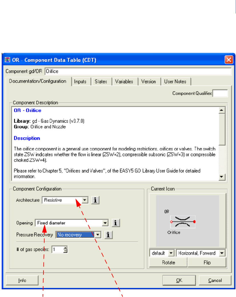
With Easy5 version 7.0 and above, and GD library version 3.0 all of these functionalities are contained within

a single component OR (OD, OW and OV have been placed in the Obsolete group):

Figure 2 Selection Parameters in the OR-Orifice Component

Choose between Fixed

Diameter and Variable Area

Choose between Resistive

and Storage/Resistive Area

Main Index

Gas Dynamics Library User Guide

Network Considerations

The following types of configurations are common to many components in the GD library:

Architecture- The user may choose between Resistive and Storage/Resistive architectures for the OR orifice

and most valve components. Choosing the Storage/Resistive architecture activates pressure and temperature

states for upstream volume(s).

The user may choose between Storage and Storage/Resistive architectures for the volume components CS,

NO, VY. Choosing the Storage/Resistive configuration activates flow constraint states that must be

initialized, and requires the use of the RADAU54 integrator for simulation.

There are advantages to each type of architecture. Choosing Storage/Resistive architectures for all

components usually simplifies the model-building process, but the additional model states results in increased

CPU times and, for volume components, no choice of integrators- RADAU54 must be used. Choosing

Resistive (for valves and orifices) and Storage (for volumes) architectures may result in more time spent in

determining the optimal combinations of component configurations to connect, but the resulting model will

have a minimal number of states, often allow a choice of integrators, and run most efficiently. Experience has

shown that the extra investment of time that may required to build a model with a minimum number of states

will be returned in the form of decreased simulation run time, hence the default configuration for most

components is Storage (for volume components) or Resistive (for orifices, valves and flow resistances.

Formulation- All Storage and most Storage/Resistive components allow the user to select between Explicit and

Implicit formulations. (Storage/Resistive volumes always use the Implicit formulation). This allows the user

to choose between a formulation that allows either of the Gear algorithms to be used (Explicit) and a

formulation that is optimal for (and requires) RADAU54 (Implicit).

We recommend that the Explicit formulation be used, in conjunction with the BCS-Gear or Stiff Gear

algorithms, whenever possible. However, some circumstances require that RADAU54 be used:

 Modeling chemical reactions with CR or ER

 Modeling a compressor based upon polytropic efficiency with CP

 Modeling laminar leakage from an actuator volume with LL

 Using Storage/Resistive configurations of volume components such as CS, NO or VY

 Coupling a GD library model with a mechanical motion model containing constraints

If it is necessary to use the RADAU54 integrator then we recommend that the Implicit formulation be used

for all components in the model, which will minimize the CPU time for simulations with this integrator, and

may make a difference between success or failure of the analysis. Models containing the transient momentum

pipe PC are particularly sensitive to formulation- simulations with RADAU54 have been observed to fail (due

to floating-point errors) when Explicitly formulated pipes are contained within the model.

The Explicit and Implicit formulations (when both are defined) are always physically identical, and differ

only in how the problem is numerically solved. For example, consider the mass and energy balances for an

ideal gas in an open, fixed volume with one inlet and one exit:

- V

-–

V– ρVc

–

max w

0,()c

T–()k

+[]min w

0,()c

T–()k

+[]q

+–

Main Index

Chapter 1: Overview

Component Types

This is a system of two equations and two unknowns ( and ), which in compact matrix notation can be

expressed as E = f(s, u, t) where E is the 2x2 matrix on the left-hand-side, is the 2x1 rate vector on the

left-hand-side, and f is 2x1 vector on the right-hand-side of the equation. For an explicitly formulated

component this equation is solved at each call to the model from the integrator: = E

-1

An implicitly formulated component takes advantage of the capability of RADAU54 to directly integrate

equations of the form E = f(x, u, t). This conserves the CPU time, and avoids the possible numerical

difficulties associated with explicitly solving the matrix equations for . The syntax for doing this is described

in Chapter 13 of the Easy5 User Guide, “Implicit Modeling.” Examples of this syntax can also be found by

examining any of the GD library components (Library > Examine) that have the option of an implicit

formulation.

Component Types

Actuators

Double chamber linear actuator

Single chamber linear actuator

One-Dimensional Body Dynamics

Single moving mass with hard limits and friction

Two adjacent masses with hard limits and friction

Two interlocking masses with hard limits and friction

Two concentric masses with hard limits and friction

Boundary Conditions

Inlet orifice (pressure specified)

Inlet valve

Ram air inlet.

Boundary flow resistance

Tabulated mass flow parameter

Variable downstream: pressure and temperature specified

Variable upstream: pressure and temperature specified

Forces and body dynamics

Forces and/or volumes from dimensions and pressure

Main Index

Gas Dynamics Library User Guide

Component Types

Solenoid Force

Spring force

Spring stop

Sum of forces

Viscous damping

Compressor, Fan & Turbine

Compressor, based upon map of corrected flow

Compressor, based upon map of polytropic efficiency

Fan, based upon performance map

Simple shaft

Turbine, based upon map of corrected flow

Directional Control Valves

Five-way three position DCV

Four-way three position DCV

Three-way two position DCV

Heat Exchangers

Primary gas: single pressure state, discretized temperature array

Primary gas: discretized temperature and pressure vectors

Secondary gas: single pressure state, discretized temperature array

Secondary gas: discretized temperature and pressure vectors

Gas/gas heat exchanger: based upon efficiency map

Gas/liquid heat exchanger: based upon efficiency map

Minor Losses

Circular pipe bend

Converging branch

Diverging branch

Elliptical bend

Gradual contraction

Offset or compound bend

Rectangular bend

Main Index

Chapter 1: Overview

Component Types

Sudden contraction

Screen or grid

U-bend

Z-bend.

Miscellaneous

Filter

Gas properties

Additional gas makeup

Orifice area vs. position

PI Controller with hard limits

Pipe insulation with heat transfer to ambient

Rupture disk area

Water/gas separator.

Nodes and volumes

Cabin- with mass and energy sources/sinks.

Node- General purpose, can be configured as Storage or Storage/Resistive

Variable volume-can be configured as Storage or Storage/Resistive

Orifice and Nozzle

Converging-diverging nozzle

Fixed diameter orifice (resistive)

Fixed diameter orifice with upstream volume (storage/resistive)

Variable area orifice (resistive)

Variable area orifice with upstream volume (storage/resistive)

Pipes, lines and tubes

Discretized (finite difference) pipe with transient momentum and heat transfer

Method of characteristics pipe with transient momentum and heat transfer

Resistive pipe or annulus with heat transfer

Flow resistance based upon K-value or sDp vs. flow

Generalized flow resistance with multiple heat sources

Laminar leakage through an annulus

Main Index

Gas Dynamics Library User Guide

Equations of State in the Gas Dynamics Library

Sensors

Flow sensor

Pressure sensor

Temperature sensor

Thermal Analysis

Thermal node (diffusive or algebraic)

Thermal conductance (linear and/or radiation conductance)

Heat input summer

Pipe insulation with H.T. to ambient

Valves (each configurable as Resistive or Storage/Resistive)

Check valve- Includes simple and piloted operation.

Pressure regulating valve

Pressure relief valve with dynamic response

Simple Valve - Models the following types of valves: butterfly, gate and globe valves.

Equations of State in the Gas Dynamics Library

The equation of state that is used in the model is specified in component GP. If there is more than one gas

makeup then the equation of state can be specified for each gas makeup in the GM component(s).

The ideal gas option is the default, and will always result in the shortest simulations, hence we recommend

its use as long as it is physically realistic for your system. The gas density is given by

where ri is the species density, P

is the species (partial) pressure, M

is the species molecular weight, R is the

molar gas constant and T is the absolute temperature. The molar heat capacity, viscosity and thermal

conductivity are functions of temperature only, and correlated by cubic power series. A mixture heat capacity

is assumed to be a linear combination of the species heat capacities:

Important: Only one tabulated gas can be stored in memory during an analysis, so if there are

multiple gas makeups in your model then the option of a tabulated gas can be used in

only one of the gas makeups. If this equation of state option is specified for more than

one gas makeup, then it will only be applied to the make-up with the lowest index.

The Lee-Kestler equation of state will be used for the other tabular gases.

-----------

Main Index

Chapter 1: Overview

Guidelines for Building and Analyzing GD Models

A mixture viscosity or thermal conductivity is calculated with the following mixing rule (3):

where

Guidelines for Building and Analyzing GD Models

Connecting Components

Always use the port option rather than the default when making fluid stream connections between

components with more than one inlet or exit port; otherwise, a default connection is all that is required.

Although a single connection line is displayed in the schematic between connected components, the line will

usually represent two to eight connected quantities. CLICK-M to examine the connection lines to verify all

expected connections have been made.

For bidirectional connections, bidirectional arrowheads are displayed as a default in the schematic. You can

modify the setup file for your Easy5 installation if you prefer single arrowheads. See Chapter 5 of the Easy5

User Guide for more details.

System Size

When developing a large model, usually the most efficient approach is to start small and expand. Develop

subsystem models first and find a steady-state operating point for each subsystem. Then merge and analyze

subsystems sequentially until the total system is developed. Use the Copy a Group utility to merge subsystem

models very efficiently.

Data Entry

You usually enter individual component data into a component’s on-screen data table. Component data

consists of tables, parameters, and initial conditions (for state variables). This data should represent the

primary database configuration for each component. Off-nominal data should not be entered into the

component data table but instead through temporary settings files or auxiliary input files specified at analysis

setup time.

pi,



mix

j 1 n,=



--------------------------

i 1 n,=



-------

------





12⁄–

----





12⁄

------





14⁄

Main Index

Gas Dynamics Library User Guide

Guidelines for Building and Analyzing GD Models

Error Controls

The GD library requires tight error controls in order to obtain physically realistic results. The following error

controls have been found to work in the models tested to date, and are the defaults for most of the GD library

components:

Occasionally, tighter error controls need to be used for a successful analysis. A convenient feature for

implementation of tighter error controls throughout a model is in the “General” tab of Analysis Settings

panel. There is a cell labeled “Multiply Error Controls (for continuous states) By”. All error controls for

continuous states are multiplied by this value (the default is 1). As an example, if a value of 0.1 is entered,

then all Error Controls for continuous states in the model will be tightened by a factor of 10.

There have also been instances where the error controls could be safely loosened with a significant decrease

in simulation CPU time, and the “Multiply Error Controls (for continuous states) By” feature may also be

used to loosen all the error controls in a model. However, we recommend that no error control for any

continuous state exceed 0.001, so caution should be used when taking advantage of this feature.

Model Operating Points

The operating point for an Easy5 model consists of numerical values for each state in your model (the state

vector), and the value of time (pertinent if your model includes time-dependent data). Easy5 allows you to

save operating points by user-specified filenames. These files can represent system steady-states at different

ambient conditions, model configurations, and others.

Load any operating point file into your model with the Options > Restore Operating Point menu. See the

section on auxiliary input files in the Easy5 Users Guide for other options to load model data.

Note: The Easy5 default value for some state variable initial conditions is not a good value for

pressures and temperatures. Initialize all primary state variables with as good an estimate as

you have.

Table 1-3 GD Library Error Control Defaults

State Error Control

Fluid Pressure 1.0e-07

Fluid Temperature 1.0e-08

Fluid Velocity 1.0e-06

Flow 1.0e-06

Switch States 1.0e-08

Most Other States 1.0e-06

Main Index

Chapter 1: Overview

Guidelines for Building and Analyzing GD Models

Steady-State Analysis

Systems modeled by the GD library are usually highly nonlinear. To find steady-state, Easy5 uses a modified

Newton-Raphson technique that uses the system Jacobian formed by a linearization of the nonlinear model.

The success of the steady-state operation for highly nonlinear systems can be very dependent on the user-

defined initial state vector.

Each valve and orifice component contains a switch-state that indicates the flow regime (molecular, viscous,

compressible or choked). Provision has been made for estimating these switch states during the calculation of

initial conditions. The estimates are based upon, and are exact for, perfect gas conditions. This estimation can

be enabled by setting the ICC parameter in the GP component to 1.

If your steady-state or transient analysis fails, execute a linear model generation analysis by selecting the

Analysis > Nonlinear > Linear Model Generation menu. This will print the Jacobian matrix and its

eigenvalues.

Examine the matrix and eigenvalues for unusual data, such as any of the following:

 Extremely large numerical values. This could indicate poor scaling or an ill-posed system.

 A row or column whose elements are all the same or nearly the same. This usually means the user has

included FORTRAN code that uses a local variable for memory or that calculated quantities are

being used before they are calculated or redefined.

 Many eigenvalues with large positive real parts (usually indicates a model with incorrect connections

or bad data).

If a model contains actuator components (AC or AX) or mass dynamics components (PM or TM), it often

helps to find a steady-state with the position states frozen and save the resulting state vector. Use this saved

state vector as the initial operating point for a second steady-state analysis with one or more position states

activated, and repeat until a valid steady-state operating point is obtained.

Often some type of control action, that is, flow rate control, temperature control, or pressure control, is

included in a model. It is usually a good idea to first find steady-state for a subsystem with the controls frozen

and to save the resulting state vector. Then, using the saved state vector as the set of initial conditions for the

next steady-state, activate one controller and find steady-state, again saving the state vector. Repeat the

Note: The Easy5 Steady State solver will usually not work for the following types of models: 1)

models that include the Method of Characteristics (PX) pipe component, 2) models of

multispecies (variable composition) fluids. For these types of models you should simulate to

a steady-state condition using one of the stiff system integrators (Stiff Gear, BCS Gear or

RADAU54). When using a stiff system integrator as a steady-state solver you need to ensure

that all function generator have constant outputs that correspond to the initial time for

subsequent analysis.

Note: These results may not be relevant if your system has unreasonable initial condition values.

Main Index

Gas Dynamics Library User Guide

Guidelines for Building and Analyzing GD Models

sequence as you activate all controllers. Remember, proportional controllers have no states to freeze, but you

can set the proportional gain to zero to fix the valve position.

Occasionally you may find that a system that includes a controller with integral type control (zero steady-

state error) fails to converge and the resulting state vector is numerical nonsense. Your system as defined may

simply not have a steady-state solution at the set point or points you have requested. Relaxing the set point

or points may help.

If steady-state analyses persistently fail to converge, you can often obtain a better set of initial conditions by

performing a short simulation (with no forcing functions) and saving the state vector that exists at the end of

the simulation.

Another strategy for determining a steady-state operating point, applicable only for models that can handle

reverse flow (most GD and HC components) is to start with a trivial solution- a system at uniform

temperature and pressure and zero flow. Use steady-state analysis to then relax the boundary conditions to

the desired values and obtain the desired solution. Finally, it is important to realize that volumes with only

one input or one output, such as a blowdown tank, do not have a non-trival steady state. Often one will know

the initial conditions apriori, so that steady-state analysis is not necessary. If steady-state analysis is necessary

for such a system, then one must first freeze the pressure and temperature states for the blowdown tank.

References

1. A.H. Shapiro, The Dynamics and Thermodynamics of Compressible Fluid Flow, 1, Ronald (1953).

2. B.W. Andersen, The Analysis and Design of Pneumatic Systems, Wiley (1967).

3. R.B. Bird, W.E. Stewart and E.N. Lightfoot, Transport Phenomena, Wiley (1960).

Main Index

Chapter 2: Tutorial

MSC Nastran Implicit Nonlinear (SOL 600) User’s GuideGas Dynamics Library User Guide

Tutorial



Introduction 22



The Conceptual Model 22



Creating the Easy5 Block Diagram 22



Determining an Initial Operating Point 32



Simulating the System 35



Using Easy5 to Analyze a More Complex System 39

Main Index

Gas Dynamics Library User Guide

Introduction

This tutorial is designed to familiarize you with some of the special considerations needed to model and

analyze gas flow with Easy5. Before beginning this tutorial, you should have installed Easy5 on your

computer and completed the tutorial section (Chapter 3, “Quick Tutorial”) in the Easy5 User Guide. You

should also have read Chapter 1: Overview of this user guide. It is assumed that you are already familiar with

the use of Easy5 to model and analyze simple systems.

The tutorial will guide you through the construction and analysis of a pneumatic system model. During this

process, several common mistakes that can be made will be pointed out. The tutorial may take two or three

hours to complete. We recommend that you set aside this time and work entirely through it. There are some

sections, marked lemmas, that illustrate important points but do not need to be completed to finish the

tutorial model.

The Conceptual Model

Pneumatic systems require some sort of power supply to do useful work. They may either require power input

(a compressor) or be statically charged with a reservoir of high pressure gas (such as a blowdown tank). For

the purposes of this example, you will select a blowdown tank as the power source. The system will be used

to power an actuator piston that is working against a load, in this case, pushing against a spring.

Such a system could be represented with the following schematic:

Figure 1 Tutorial System Schematic

Creating the Easy5 Block Diagram

An Easy5 block diagram is constructed by adding Easy5 components to an on-screen schematic, and

establishing data connections between these components. The following sections explain how to add and

connect components.

Main Index

Chapter 2: Tutorial

Creating the Easy5 Block Diagram

Adding Components

To begin your model of the blowdown tank subsystem, you will need some files stored by Easy5 in a special

directory for this tutorial. To retrieve these files, first enter the command you use to run Easy5 in a command-

shell and supply the option -demos, as shown in the following example:

Before starting the tutorial, you need to copy the tutorial files by either:

1. Typing the command

easy5x -demos at a command shell prompt, OR

2. Select Start > Program Files > Easy5 2021.3 > Demos >Copy Easy5 Demo Files in Windows.

3. Type in the option gd when prompted to enter the corresponding DirName.

Step Action

1 Start Easy5.

2 Enter a new model name called BlowdownTank when the opening menu displays.

3 Select the Add button.

4 When the Add Menu displays, scroll down the top section (Libraries) until the gd - Gas Dynamics

library displays.

5 Select the gd - Gas Dynamics library.

6 Select Nodes and Volumes from the Groups Menu.

7 Before dropping the component onto the schematic, add the qualifier, TN (for tank) to name the

component NOTN.

To do this, select the component from the bottom window of the Add window. The library and

component name display in the Add Component input field as gd/NO. Type in the qualifier TN

after NO.

8 Add NOTN to the schematic. Examine NOTN by pointing the cursor at the component and

either clicking the middle mouse button once or double-clicking the left mouse button. Click on

the Configuration tab if it is not active. Use the left pull down menu, under the icon, to change the

icon from Default to One Exit Port.

9 Add a variable area orifice. Select Orifices from the Groups Menu and add the OR-Orifice and set

the qualifier to TN. Place this component to the right of the NOTN component. Examine ORTN

and click on the Configuration tab if it is not active. Use the pull down menu to change the

Opening from Fixed Diameter to Variable Area, Internal Dynamics.

10 From the Pipes and Flow Resistances group, add the PC component with the qualifier BD (for

blow-down). Rotate the icon 270o by point the cursor at PCBD, right-click and hold, and select

Rotate from the popup menu.

Then repeat the last step, but select Flip instead of Rotate.

11 Add a GP-Gas Properties component from the Miscellaneous group. GD library models must

have one and only one GP component to identify global parameters, such as the gas species that are

present.

Main Index

Gas Dynamics Library User Guide

Creating the Easy5 Block Diagram

Easy5Your schematic should look like Figure 2.

Each component is identified by a title, such as Blowdown Tank, and a name, such as NOTN. You should

edit the title of each component to match the titles used in

Figure 2. Although this is not required, it helps to

document your model. To edit the title, select each component with a hold-right mouse button. Then select

Edit Title from the pop-up menu and edit the titles to match the titles used in this tutorial.

Figure 2 Initial Easy5 model without connections

If your component names do not match the names shown in

Figure 2, you should edit them as well. For

example, the NO Node component used in this model is named NOTN. The component name is a four-

character name using the two-character component identifier, NO, followed by a two-character

alphanumeric qualifier, “xx”. The qualifier is used to insure that each component has a unique name. Easy5

assigns the qualifier by default, although you can easily change it. To change it, highlight the component,

then press and hold the right mouse button. Select Open Data Table from the pop-up menu, select the

Documentation/Configuration and change the two-character qualifier as needed to match the component

names used in this tutorial.

Making Connections: Ports and Their Significance

The node component NOTN has at least 4 Inlet ports and 4 Exit ports. Inlets are characterized as connection

points where flow entering the component is positive, while at an Exit flow exiting a component is considered

as positive. Negative flows can be considered at any port. All Inlet ports are equivalent for component

NOTN, as are all Exit ports. However, this is not always true for other component in the GD library.

The port connection concept in Easy5 is very useful as it enables the communication of many items of fluid

information (flow rate, pressure, temperature, etc.) with a single action between adjacent components. (See

Network Considerations".)

Main Index

Chapter 2: Tutorial

Creating the Easy5 Block Diagram

To perform the default port connection between the NOTN and ORTN components, simply Click-R on

NOTN, then Click-R on ORTN. To specify a particular Inlet port or Exit port when connecting

components that have multiple Inlets and/or Exits, follow the steps below:

Step Action

1 Select the NOTN node component.

2 Right-click and hold with the cursor hovering over the ORTN component. Select Create Custom

Connection from the Component Connection Menu.

3 Select Exit2 under NOTN Source Ports

4 Select Inlet1 under ORTN Target Ports

5 Select OK. The connection is completed; it displays in the Port Connections field.

Main Index

Gas Dynamics Library User Guide

Creating the Easy5 Block Diagram

Figure 3 Port connection table.

Expand the connection by clicking on the + sign next to Exit2.

Figure 4 Expanded Connection Specification

This is an example of a bi-directional ported connection. The quantities W_Inlet1_ORTN,

WL_Inlet1_ORTN, TR_Inlet1_ORTN and KR_Inlet1_ORTN are passed from the orifice to the node, and

Main Index

Chapter 2: Tutorial

Creating the Easy5 Block Diagram

the quantities PP_Exit2_NOTN, TF_Exit2_NOTN, KF_Exit2_NOTN, and Q_Exit2_NOTN are passed

from the node to the orifice.

To continue the tutorial, make the following connections in your model, using the default connection

method. (See the Lemma on Default versus Port Connections)

The finished schematic should look similar to Figure 5.

Step Action

6 Connect ORTN to PCBD.

Lemma

Multiple Gas Species

Gas streams of variable composition may be modeled by setting the # of Gas Species in the

configuration tab of the component data table of GP, and in each fluid flow component, to the

appropriate number. The flow W is then a vector of species flows, and PP is a vector of species partial

pressures.

If multiple species are present, but the relative amounts do not change, then you can treat the gas as a

single species, as is commonly done for air.

Component GM - Additional Gas Make-ups is used to specify the gas species if there is more than

one gas make-up. For example, a model could be formulated with one stream containing air and

another stream containing pure nitrogen. There may be up to four GM components in a model, so that

five make-up streams (the first specified by the GP component) may be modeled.

Main Index

Gas Dynamics Library User Guide

Creating the Easy5 Block Diagram

Figure 5 Blowdown Model with Connections

Entering Data into the Model

Before you begin to enter data into your model, you will have to make a key decision that globally affects

your model; the system of units used, either SI or English. You will be using English units in this tutorial.

This information is entered into the GP component. Other data in the GP component is used to specify the

gas species that are present (but not the relative amounts), the ambient temperature, the pressure if not

otherwise specified, and other parameters.

You should first read Chapter 1: Overview of this user guide and the GP - Gas Properties component data

sheet for a more complete discussion of these parameters and of make-up indices before working on this part

of the tutorial.

Follow the steps below to enter more data and continue the tutorial:

Note: Any parameters or states that are not specified in the following section should be left at their

default values.

Main Index

Chapter 2: Tutorial

Creating the Easy5 Block Diagram

Step Action

1 Examine the GP - Gas Properties component; select it with a double click.

This opens the component data table. In the Documentation/Configuration tab there is a

Component Configuration called “# of gas species”. You will leave this setting in all components

at the default value of 1, indicating that the species pressures PP and the flows W are scalars

describing single gas species.

2 Enter the following data into the GP component. The input UN is used to select the unit system,

and GAS=1 defines the working gas to be dry air. TAM sets the ambient temperature to 86

F and

PAM defines the ambient pressure to be 14.7 psia. (Some other GD library components also have

inputs for local ambient conditions. The global ambient conditions set in component GP are used

when the local conditions have not been initialized.)

In Component For Parameter . . . Input the Value . . .

GP UN English

GAS 1

TAM 86

PAM 14.7

Main Index

Gas Dynamics Library User Guide

Creating the Easy5 Block Diagram

3 Change the names of some outputs in the model to be more mnemonic. You can change them by

examining the given component, double-clicking on the name to be replaced until it is completely

highlighted, and typing the new name.

Use the names given in the table below:

4 Since all user-defined names have been supplied, and the default component dimensions have been

accepted, you can now create an executable by selecting Build > Create Executable.

Step Action

For Component...

With the Easy5 Output Name .

. .

Type the New User-Defined

Name . . .

NOTN P1 (Secondary Variables) TankPressure

TF_Exit2 (Ported Variables) Tan kE xi tTem p

ORTN ACS (Primary States) OrificeArea

W_Exit2 (Primary Variables) Tan kE xi tFl ow

TS (Secondary Variables) OrificeStaticTemp

PS (Secondary Variables) OrificeStaticPressure

VS (Secondary Variables) OrificeVelocity

MCN (Secondary Variables) OrificeMachNumber

PCBD W_Exit (Primary Variables) PipeExitFlow

TF_Exit (Primary Variables) PipeExitTemp

P1 (Secondary Variables) PipeInletPressure

Note: If there were any tables in the model, they would need to be dimensioned

before creating the executable.

Main Index

Chapter 2: Tutorial

Creating the Easy5 Block Diagram

5 While that operation is continuing in the background, enter the rest of the parameter data for this

model:

Step Action

In Component . . . For Parameter . . . Type in the Value . . .

NOTN VOL (Primary Inputs) 1000

HI (Thermal Inputs) 10

HO (Thermal Inputs) 10

AHT (Thermal Inputs) 10

MTW (Thermal Inputs) 100

TAM (Thermal Inputs) 86

ORTN ARE (Primary Input) 0.01

TimeConstOpening 2

TimeConstClosing 2

CD (Primary Input) 0.8

PCBD LEN (Primary Input) 10

DH (Primary Input) 0.2

PP_Exit (Primary Input) 100

TR_Exit (Primary Input) 86

Main Index

Gas Dynamics Library User Guide

Determining an Initial Operating Point

An initial operating point, or a set of “initial conditions,” can be determined in a number of ways:

 By knowing, a priori, the initial condition values and simply making them known to Easy5.

 By using Easy5’s Steady-State Analysis to solve for a set of initial condition values.

6 You need to initialize the pressure and state initial conditions — the starting values by entering the

following state initial conditions:

7 Enter “Blowdown System Example” in the Title field that appears when File > Properties ... is

selected.

8 Save the model (you can use the accelerator key Ctrl + S) to record the data you just entered.

Lemma

Multiple Gas Species

Gas streams of variable composition may be modeled by setting the # of Gas Species in the

configuration tab of the component data table of GP, and in each fluid flow component, to the

appropriate number. The flow W is then a vector of species flows, and PP is a vector of species partial

pressures.

If multiple species are present, but the relative amounts do not change, then you can treat the gas as a

single species, as is commonly done for air.

Component GM - Additional Gas Make-ups is used to specify the gas species if there is more than

one gas make-up. For example, a model could be formulated with one stream containing air and

another stream containing pure nitrogen. There may be up to four GM components in a model, so that

five make-up streams (the first specified by the GP component) may be modeled

Step Action

In Component . . . For State . . . Type in the Value . . .

NOTN

PP_Inlet

500

PP_Inlet

PCBD

PPS

100

TW_Wall

Main Index

Chapter 2: Tutorial

Determining an Initial Operating Point

 By calculating our own initial condition values using a customized Code component with special

code and the Initial Condition analysis.

 By integrating to steady-state using a Simulation analysis.

In this example you’re going to use Easy5’s Steady-State Analysis to locate a set of initial conditions for us.

The gd library presents some difficult problems for finding steady-state operating points. The differential

equations in pressure and temperature are coupled and nonlinear. Therefore, you may have to take some

special measures to find a stable operating point. These techniques are shown as “hints” in this section.

The GP component contains a parameter ICC that is, by default, initially set to zero. If this value is set to

unity, special code will be executed during the initial condition calculation (Calc-XIC) that precedes all

analyses, including steady-state analysis, to estimate the flow indicator switch states in all orifice and valve

throats.

This steady-state estimate, which is exact for perfect gases, is based upon the upstream and downstream

pressures, the upstream temperature, and the upstream kinetic energy. The upstream and downstream

pressure and upstream temperature are usually states (unless they come from a boundary condition) and need

to be estimated as best you can.

A convenient way to do this is to create a temporary settings file called ICCALC which contains the single

parameter ICC from the GP component. This leaves the nominal value of ICC at zero, which will be the

desired value once an initial operating point is found and saved, and simulations are performed.

To create the Temporary Settings File called ICCALC, use the procedure below:

Hint: Steady State Hint #1: Set the parameter ICC in the GP component to unity when doing a

steady-state analysis to have Easy5 estimate values for the orifice switch states.

Note: A good practice is to create Temporary Settings files to hold parameter settings for abnormal

or different conditions. In this way, the model itself retains the nominal values for the

parameters.

Step Action

1 Select the Temporary Settings File icon .

2 Select the New Temporary Settings File icon .

3 Click on the plus (+) sign next to the GP - Gas Properties component in the Model Explorer

component list so expand the GP component input list.

4 Select the ICC input name from the CDT. This copies the name and value into the lower window.

5 In the Temporary Settings Editor, change the value of ICCGP to 1.0.

Main Index

Gas Dynamics Library User Guide

Determining an Initial Operating Point

Setup and run the Steady-State analysis using the procedure below:

Steady-state analysis will solve for the final values in all states that are not frozen. However, you will be

performing transient simulation of the valve (component ORTN) opening, so you need the initial operating

point to be based upon the initial value of the valve opening (zero).

Create a second temporary settings file called FreezeOrifice. Add the state OrificeArea from the ORTN

component to the temporary settings form and freeze the state by repeatedly clicking on the “Frozen” field

value until the value of “YES” displays, as shown in

Figure 6.

Figure 6 Freeze the OrificeArea State

Add the temporary settings file FreezeOrifice to the Steady State Analysis form. Also, save the final operating

point. Set “Save Final Operating Point” to Yes, and “Save ID:” to SteadyState. Then, execute the analysis.

When the analysis completes, the steady state output data displays. The ZSWORTN state should be equal

to 4.0. If the analysis didn’t converge with this state value, recheck all the parameter values you entered in the

previous section.

If you check the eigenvalues of the model, this will be a further confirmation that the model was built

correctly. Check further down in the output listing, and note the eigenvalues.

Step Action

1 Select Analysis > Steady State to bring up the Steady State Analysis form.

2 Click on the Modifiers tab. Add the temporary settings file ICCALC to the form.

Main Index

Chapter 2: Tutorial

Simulating the System

Since there are no eigenvalues with positive real parts, the linearized system is stable at this operating point.

The lowest frequencies, on the order of 0.001Hz, dictate that you might have to run the simulation for

thousands of (simulated) seconds to reach steady state.

Three important items should be noted:

1. The steady-state analysis reports a value for the switch state ZSWORTN that indicates choked flow,

and the variable states OrificeStaticTemp and OrificeStaticPressure reflect sonic flow, even though

OrificeArea is zero, ie., the valve is completely closed. Even though the orifice velocity is non-zero, the

mass flow (OrificeVelocity * OrificeArea * density) is zero.

2. Easy5 automatically froze some states because the state matrix (the Jacobian) was singular. This was

caused, in part, because the orifice OR was complete closed, so that there was neither thermal or

hydrodynamic communication through the orifice.

3. Since the valve is closed, and there is no flow, it is easy to know the initial conditions for this problem.

This is typical for blowdown problems. For this particular problem the main value of the steady-state

analysis is the solution for the orifice switch state.

Simulating the System

1. Open the Simulation Data form by selecting Analysis > Simulation. Enter the data and set up the

plots as shown in

Figure 7, verifying the following values:

• Stop Time = 15

• Time Increment= 0.01

• Int. Method= BCS Gear

Table 2-1 Eigenvalues

MODE REAL IMAG

1 0 0

2 -8.996997 x 10

-7

3 -1.924552 x 10

-6

4 -8.361847 x 10

-4

5 -1.55672 + - 122.734

6 -1.83213 0

7 -10.7690 0

8 -26.5489 0

Note: The calculated values you get may be a little different from the values indicated in this

document. This is due to differences in numerical precision used by various computers.

Main Index

Gas Dynamics Library User Guide

Simulating the System

2. In the Plotting tab, set up 4 displays:

• Display 1: plot OrificeStaticPressure and TankPressure as an overplot (click on the plus (+) sign

next to Advanced to reveal the Overplot option).

• Display 2: plot PipeExitTemp and TankExitTemp as an overplot.

• Display 3: plot PipeExitFlow and TankExitFlow as an overplot

• Disply 4: plot OrificeVelocity and OrificeMachNumber

Execute the simulation. When the plotted results appear, they should look similar to the plots shown in

Figure

and Figure 8.

Main Index

Chapter 2: Tutorial

Simulating the System

Figure 7 Results of Initial Simulation

Blowdown System Example

0246810

100

200

300

400

500

Model: BlowdownTank, Runid: simulation, Case: 1, Display: 1. 23-JAN-2001, 15:47:05

TIME

OrificeStaticPressure,TankPressure

OrificeStaticPres

TankPressure

0 2.5 5 7.5 10 12.5 15

-40

-20

100

TIME

PipeExitTemp,TankExitTemp

PipeExitTemp

TankExitTemp

Main Index

Gas Dynamics Library User Guide

Simulating the System

Figure 8 Results of Initial Simulation (contin.)

Blowdown System Example

0246810

-0.01

0.01

0.02

0.03

0.04

0.05

0.06

Model: BlowdownTank, Runid: simulation, Case: 1, Display: 3. 23-JAN-2001, 15:47:05

TIME

OrificeFlow,PipeExitFlow

OrificeFlow

PipeExitFlow

Blowdown System Example

0246810

0.98

1.02

1.04

1.06

1.08

1.1

0246810

960

980

1000

1020

1040

1060

Model: BlowdownTank, Runid: simulation, Case: 1, Display: 4. 23-JAN-2001, 15:47:05

TIME

OrificeVelocity

TIME

OrificeMachNumber

Main Index

Chapter 2: Tutorial

Using Easy5 to Analyze a More Complex System

Before starting this section, copy the operating point obtained from the steady-state analysis into your model

by selecting Options > Restore Operating Point and specifying the SteadyState operating point.

In this part of the tutorial, we are going to connect the power supply you just built to a linear positioning

system and simulate the combined system performance.

Start by saving the BlowdownTank model and opening the model PneumaticLinPos in a directory under

your current working directory called “Pneumatic/PneumaticActuator”. This directory was created as the

result of the “-demos” command you did to start the tutorial. This model is shown in

Figure 9.

Figure 9 PneumaticLinPos demo model

The PneumaticLinPos model represents a linear positioning system. A constant pressure supplied to the 5-

way-valve powers the dual-chambered actuator. The actuator is positioned with a proportional/integral

controller, which compares the command signal to the actuator position and controls the valve spool

movement. You can look at the results of a simulation by selecting Analysis > Open Plotter >

PneumaticLinPos.baseline.ezrpd.

The components in the BCUP submodel are used to provide a constant pressure to the servovalve, but you

will be connecting the BlowdownTank to the servovalve inlet. Delete the BCUP submodel components. You

might want to Zoom Out the schematic now to make room for the Blowdown Tank.

Spring Force

Upstream BC's

Submodel

Directional Valve

4-Way

Actuator

(Twin-chambered)

Valve driver

PI Controller

Submodel

CONTROL

Downstream

BC's Submodel

CommandedValvePosition

Two tabular

functions of time

ValveCommandOutputSignal

Feedthrough

SetPoint

Select "Model Info"

above for details

Feedthrough

PistonPosition

Main Index

Gas Dynamics Library User Guide

Using Easy5 to Analyze a More Complex System

Select Edit > Copy Group From . . . Select the BlowdownTank model you just built and saved, and place it

below the existing components.

When importing the Blowdown Tank Model, Easy5 detects that some user-defined names are already used,

and brings up a window to change the name. Select the apply button to let Easy5 automatically select new

names.

The completed schematic is shown in

Figure 10. You will need to move your components and connections

around, select the appropriate icons, and add the TI component from the Interactive Simulation (IS) library

to get your schematic to look like this one.

Figure 10 Completed Combined Model

Since the pipe pressure of 100 psia matches the BCUP supply pressure, a steady-state analysis is not required.;

Bring up the simulation settings panel and enter a Start Time of 0, a Stop Time of 30, and a

Time Increment 0.01. Enter SteadyState for the initial operating point.

Select the Plotting tab of the simulation settings panel. Some displays are already defined (because an analysis

settings file accompanied the demo model), but modify the plot settings and follows::

Display

2 OrificeStaticPressure, TankPressure

Spring Force

Directional Valve

5-Way

Node

Actuator

(Twin-chambered)

Valve driver

PI Controller

Submodel

CONTROL

CommandedValvePosition

Orifice

Pipe (Discretized

with Heat Transfer)

Two tabular

functions of time

SetPoint

PistonPosition

ValveCommandOutputSignal

Simulated and

accumulated CPU times

PLPwBD(9)

Main Index

Chapter 2: Tutorial

Using Easy5 to Analyze a More Complex System

Execute the simulation and the results should match Figure 11 and Figure 12.

3 OrificeStaticTemp, TankExitTemp, PipeExitTemp

7 PipeExitFlow, TankExitFlow

8 OrificeVelocity, OrificeMachNumber

Display

Main Index

Gas Dynamics Library User Guide

Using Easy5 to Analyze a More Complex System

Figure 11 Results from simulation of full model

Simulation of Pneumatic Actuator Control System

0 5 10 15 20 25 30

-3

-2

-1

Model: PLPwBD, Runid: simulation, Case: 1, Display: 1. 26-MAR-2003, 20:13:48

TIME

BumplessSetPoint,PistonPosition,SetPoint

BumplessSetPoi

PistonPosition

SetPoint

Simulation of Pneumatic Actuator Control System

0 5 10 15 20 25 30

100

200

300

400

500

Model: PLPwBD, Runid: simulation, Case: 1, Display: 2. 26-MAR-2003, 20:13:48

TIME

PressureStaticExtendVol,PressureStaticRetractVol,

PressureStaticEx

PressureStaticRe

OrificeStaticPres

TankPressure

Main Index

Chapter 2: Tutorial

Using Easy5 to Analyze a More Complex System

Figure 12 Results from simulation of full model

Simulation of Pneumatic Actuator Control System

0 5 10 15 20 25 30

-0.01

0.01

0.02

0.03

Model: PLPwBD, Runid: simulation, Case: 1, Display: 7. 26-MAR-2003, 20:13:48

TIME

PipeExitFlow,TankExitFlow

Simulation of Pneumatic Actuator Control System

0 5 10 15 20 25 30

0.2

0.4

0.6

0.8

0 5 10 15 20 25 30

200

400

600

800

1000

1200

Model: PLPwBD, Runid: simulation, Case: 1, Display: 8. 26-MAR-2003, 20:13:48

TIME

OrificeVelocity

TIME

OrificeMachNumber

Main Index

Gas Dynamics Library User Guide

Using Easy5 to Analyze a More Complex System

This completes the tutorial. The following chapters contain the detailed theory and usage suggestions for

many of the component groups in the Easy5 Gas Dynamics Library. Components not described in these

chapters are described in detail in the Configuration/Documentation tab of their respective Component Data

Tables.

Main Index

Chapter 3: Frequently Asked Questions

MSC Nastran Implicit Nonlinear (SOL 600) User’s GuideGas Dynamics Library User Guide

Frequently Asked Questions



Frequently Asked Questions 46

Main Index

Gas Dynamics Library User Guide

Frequently Asked Questions

Q. I have a step function generator connected to an orifice diameter, to simulate a valve opening at a certain

time.. The simulation fails at the step time.

A. Never, ever connect a function generation component directly to an orifice diameter or area, or to a valve

area. Always connect through a dynamic model that will smooth the orifice area change, such as a lag

component or a mass-dynamics model. It is both physically unrealistic and numerically destabilizing for an

orifice or flow area to change in a non-smooth fashion. While the change may be very rapid to human

perception, it is nevertheless always smooth.

Q. My transient analyses run very slowly. Why?

A. Possible reasons include:

1. Your initial operating point is physically unrealistic or contains large artificial transients, causing the

variable-step integrator to take very small time-steps at the start of the analysis.

2. You have “short, fat” pipes in your model. An extreme example (but an actual example from a user)

would be a pipe that is 1 inch long and 6 inches in diameter. The pipe inlet pressure (a state) is

physically indistinct from the downstream pressure (also a state), but a variable-step integrator will

work very hard to resolve the imagined difference, taking very small step sizes that result in long

simulation times.

3. The are two small volumes in your model separated by a small fluid resistance, such as a large diameter

orifice. The volume pressure states are then physically indistinct, but a variable-step integrator will

work very hard to resolve the imagined difference, taking very small step sizes that result in long

simulation times.

4. There are one or more very small explicitly formulated volumes in your model. The pressure and

temperature rates are inversely proportional to volume, so a very small volume will result in amplified

transients, and the variable-step integrator will take very small step sizes.

In principal, an implicitly-formulated volume simulated with the RADAU54 integrator will not have

this limitation, so that may be worth a try.

5. One or more mass-dynamics components (poppet or spool masses) are rapidly bouncing off of their

hard limits. A switch-state transition occurs each time a hard limit is encountered, and if switch-state

transitions are occurring very frequently then the simulation may run much slower than it would if

the switch-state transitions were not occurring.

These types of problems are most readily diagnosed with the “Print Detailed Diagnostics (this run only)”

feature. However, do not allow your analyses to run for a long time with this feature activated- that will lead

to unmanageably large output files. General Purpose Library component II can also be used to activate

Detailed Diagnostic- it is especially useful if you want to activate the detailed diagnostics at some point after

the simulation start time.

Main Index

Chapter 3: Frequently Asked Questions

Frequently Asked Questions

Q. My simulation fails with the message

“*** FATAL ERROR *** Integration step size has been reduced to 1.00000000E-16, and the integration

algorithm is still failing. Problem appears unsolvable with given input.

or a similar message.

A. See the previous Q & A. This is just an extreme case of a variable step integrator step size becoming so

small that it is, within the precision of real*8 arithmetic, zero. So the integrator just gives up.

Q. My simulations ran great (fast) when I was using the Ideal Gas model, but are much slower when I use

one of the non-ideal gas models.

A. That is not unexpected. One strategy for dealing with this issue, useful if the ideal gas model is “close” to

reality, is to first test your preliminary designs with the ideal gas model.

Q. I need a tabulated gas that is not currently installed with Easy5. Can we get that?

A. The tabulated gases are generated from the NIST Refprop 8 program. In principle, we can provide

tabulated properties for any fluid that is included with NIST Refprop 8. Please send your request to

[email protected].

Q. What are the limits of the built-in Lee-Kestler correlation for non-ideal gases?

A. That depends upon the gas. This maximum pressure for this correlation is 10 times the critical pressure,

and the minimum temperature is 0.3 times the critical temperature. So the answer depends upon the critical

properties of the gas you are modeling. The answer also depends upon the polarity of the gas- L-K is

recommended only for non-polar gases- it should never be used to model pure water vapor. Krypton is one

of the model gases for this correlation, so L-K is expected to be a very good model for this and other noble

gases, with the exception of helium.

Q. My valve or variable-area orifice is completely closed, but the output indicates a non-zero velocity? How

could that possibly be:?

A. Velocity and flow area are independently calculated. If the valve is closed, then the calculated velocity is

the velocity that would exist if there was any flow area. This method is used because the switch state that

indicates the flow regime (linear, compressible non-choked or choked) will need to have the correct value

when the valve does open, and because the switch state value depends upon the velocity.

Q. Steady-state analysis does not converge. What did I do wrong?

A. If you have a Method of Characteristics pipe component, or if you are modeling multiple gas species

(variable composition) then the steady-state solver probably will not work, and you should try using one of

the variable-step integrators as your steady-state solver- see the previous section on steady-state analysis.

Otherwise it is usually possible to get the steady-state solver to converge- see the tips and strategies in the

previous section on steady-state analysis.

Main Index

Gas Dynamics Library User Guide

Frequently Asked Questions

Q. I'm getting a negative value for the outlet kinetic energy from an orifice when the Lee-Kestler equation of

state. It would seem that both Tr and Pr are within the acceptable limits for using Lee-Kestler. What is going

on there.?

A. When the flow is choked and a non-ideal gas is being modeled, KF_Exit2 and KR_Inlet1 are carrying

additional information. Whereas

1. enthalpy is a function of pressure for a non-ideal gas

2. PS_OR is higher than the downstream pressure

3. the component downstream of the orifice has no information about PS_OR

the output of OR must contain some information that adjusts the output enthalpy to the downstream

pressure. The way we chose to do that was to set

KF_Exit2_OR = 0.5*VS_OR**2 - H(TS_OR,PP_Exit2_OR) + H(TS_OR,PS_OR)

We chose to do it this way rather than add an extra ported output for what seemed to be an “outlier” case.

Main Index

Chapter 4: Nodes and Volumes

MSC Nastran Implicit Nonlinear (SOL 600) User’s GuideGas Dynamics Library User Guide

Nodes and Volumes



Introduction 50



Formulation and Terminology 50



Fundamental Equations 50



Switch State Rate Calculation 53



Guidelines for Component Selection 53



References 54

Main Index

Gas Dynamics Library User Guide

Introduction

This section discusses the components in the Nodes and Volumes group of the GD library. Mathematical

models of volumes are also important to some components in the Orifices, Valves, Heat Exchangers, Pipes

and Directional Control Valves group.

Formulation and Terminology

Rigorous models of compressible gas dynamics must consider variations in gas density and the gas kinetic

energy. Classical compressible fluid flow treatments accomplish this by defining stagnation quantities such as

stagnation temperature, pressure and density.

The composition of multi-species gases is modeled through the use of partial pressures and species flow rates.

The partial pressure P

of a gas is defined as P

= Y

P where the gas phase mole fraction of species k is

where n

is the number of moles of species k. For a single-species gas, the static pressure and species partial

pressure are the same.

Depending on the context, the term “total pressure” can have two different meanings:

1. Stagnation pressure, OR

2. The sum of the species partial pressures, which is actually the static pressure.

The term total pressure will always be the sum of the species partial pressures in the Gas Dynamics Library User

Guide. The term stagnation pressure will be used where needed. Similar considerations apply to the terms

total density and stagnation density.

Fundamental Equations

Equation of State

The parameter PRP in the GP component is used to select the equation of state. If PRP is set to unity, the

ideal gas law P = ρRT is used in gas components to calculate density and other fundamental relationships. If

PRP is set to two, the gas law P = ZρRT is used, with the compressibility factor Z given by the Lee-Kestler

correlation (1, 2). If PRP is equal to three, Easy5 will search for a set of user-defined functions to calculate

the gas properties. A template for writing a set of user-defined functions is given in

Appendix A - Gas Properties.

If PRP is equal to 4, then built-in tables are used.

Equations of Continuity- Non-condensible gas species

The material balance for a non-condensible gas species j is



------------

Main Index

Chapter 4: Nodes and Volumes

Fundamental Equations

Expressing the species density rate in terms of the state variables T and p

leads to (there is one of these

equations for each species i:

Equations of Continuity- Condensible gas species

The material balance for the condensible species c is

Expressing the species density rate in terms of the state variables T and p

leads to:

The time derivative of total volume is an input to the variable volume components VX and VY, and is zero

for the other Nodes and Volumes components. The time derivatives of the gas and liquid volumes are given

by:

Condensation Rate

Mass transfer model- The mass transfer model assumes that condensation or evaporation occurs at the

container wall and is limited by diffusion of the condensible species through the non-condensible species, so

that the condensation rate is

dρ

--------

in j,

out j,

– ρ

–=

(4-1)

∂

-------





, kj≠,



∂

T∂

-------











in i,

out i,

– ρ

–=

(4-2)

dρ

cg,

-------------

dρ

cl,

------------

+ w

in c,

out c,

– ρ

cg,

cl,

––=

(4-3)

cg,

∂

------------





, ki≠,



cg,

∂

T∂

------------











cl,

∂

p∂

-----------





cl,

∂

T∂

-----------











in c,

out c,

– ρ

cg,

cl,

––=

(4-4)

cl,

---------

cl,

-----------

cl,

∂

p∂

-----------





cl,

∂

T∂

-----------











–=

(4-5)

–=

Main Index

Gas Dynamics Library User Guide

Fundamental Equations

where k

is the mass transfer coefficient (analogous to the heat transfer coefficient), A

is the heat transfer

area (assumed equal to the mass transfer area), the subscripts g and w respectively refer to the bulk fluid and

the container wall. , where p

is the condensible species pressure, p

is the sum of all

non-condensible species pressures and

The mass transfer coefficient is estimated from the heat transfer coefficient by assuming that the Lewis

number (h/kmCp) is unity, which is true for air/water gas mixtures, but not true in general (3).

Bulk condensation model- The bulk condensation model can be used for gas mixtures that include water vapor

or for pure steam. The condensation rate is assumed proportional to the bulk supersaturation:

where E

is the proportionality coefficient.

The relation between the condensate droplet surface area and the condensate mass is modeled by the factor:

where is a minimum value (if were zero then condensation could not be initiated).

Equation of Energy

The total energy balance for a stagnant volume is

The term is simply equal to -1 for an ideal or perfect gas.

cg,

cw,

–()=

(4-6)

cg,

§=

cw,

sat

()

sat

()–

----------------------------

sat

()–[]max m

ε,(){}

0.67

(4-7)

max m

ε,(){}

0.67

ρc

----------

–





---

ρ∂

T∂

------





+ w

h–()q

++ +=

(4-8)

---

ρ∂

T∂

------





Main Index

Chapter 4: Nodes and Volumes

Switch State Rate Calculation

Each of the Nodes and Volumes components has a switch state, usually named SMC, that indicates either a

single phase or two phase mixture. This switch state is active only if 1) H

O is one of the fluid species and 2)

the GP component parameter WX is set to one. An SMC value of zero indicates a single gas phase, a value

of one indicates gas+liquid, and a value of two indicates single phase liquid (possible if and only if H

O is

the only fluid species).

Mass transfer model- The rate of the switch state SMC is given by

If none of these conditions is satisfied then dSMC = SMC.

Bulk condensation model- The rate of the switch state SMC is given by

where is the void fraction (V

/V). If none of these conditions is satisfied then dSMC = SMC. SMC or dSMC

can be equal to 2 if and only if H

O is the only fluid species.

Guidelines for Component Selection

The Nodes and Volumes group contains a general purpose node NO which can model either a fixed or

variable volume. NO can be configured as:

1. Storage: The inlet ports connect to upstream storage/resistive or resistive components, while the exit

ports connect only to downstream resistive components. This component is recommended for

general use. This architecture may be Explicitly or Implicitly formulated.

2. Storage/Resistive. The inlet ports connect to upstream storage/resistive or resistive components, while

the exit ports to downstream storage or storage/resistive components. This component connects to a

wider variety of components, which makes model building easier. This is accomplished through the

use of flow constraint states, which can complicate analysis because

1) the additional constraint states must be properly initialized and 2) only the RADAU54 integrator

can be used.

The user may choose either the mass transfer or the bulk condensation model for NO. If more than four inlet

and four exit ports are need the user may activate the Extra Ports configuration, allowing 28 inlet ports and

28 exit ports.

dSMC

1 , if SMC 0= and w

lin,

lex,

+–0>

0 , if SMC 1= and w

lin,

lex,

+–0< and m

0≤







dSMC

0 , if SMC 1= and w

lin,

lex,

+–0< and m

0≤

1 , if SMC 0= and p

sat

()>

1 , if SMC 2= and p

sat

()<

2 , if SMC 1= and p

sat

()> and ϕ 0=











Main Index

Gas Dynamics Library User Guide

References

This group also contains a cabin model CS which can be configured as:

1. Storage: The inlet ports connect to upstream storage/resistive or resistive components, while the exit

ports connect only to downstream resistive components. This component is recommended for

general use. This architecture may be Explicitly or Implicitly formulated.

2. Storage/Resistive: The advantages and disadvantages of the storage/resistive NO component also

applies to the storage/resistive CS component.

NO also has ported inputs for volume and volume derivative, and can be used to model a variable volume.

To ensure that conservation of mass is enforced the user must ensure that these two inputs are consistent with

each other. Component CD, from the Forces group, may be used to calculate the volume and volume rate

from the position and velocity of a moving mass.

All Nodes and Volumes components, except for CS, use the bulk condensation model. The CS component

models a cabin volume, and is different from the NO component in only two ways:

 It has two different heat/mass transfer surfaces (wall and equipment), with two corresponding heat

load inputs, instead of a single surface.

 It uses the mass transfer model of moisture condensation.

The actuator components AC and AX (from the Actuators group) also contain variable volume models. Each

actuator volume has two inlet ports and two exit ports so that the volume can also function as a junction or

manifold.

References

1. B.I. Lee and M.G. Kestler, AIChE J., 21, p. 510 (1975).

2. R.C. Reid, J.M. Prausnitz and B.E. Poling, The Properties of Gases and Liquids, 4th Ed., McGraw-

Hill, New York (1987).

3. R.E. Treybal, Mass Transfer Operations, 3rd Ed., McGraw-Hill, New York (1980).

Main Index

Chapter 5: Orifices and Valves

MSC Nastran Implicit Nonlinear (SOL 600) User’s GuideGas Dynamics Library User Guide

Orifices and Valves



Introduction 56



Fundamental Equations 56



Orifice flow regimes 56



Solution of the orifice equations 57



Switch State Rate Calculation 58



Valve/Duct Area Models (Components VD and VI) 59



Poppet Valve Area (Component PA) 63



Component Selection- Orifices 63



References 63

Main Index

Gas Dynamics Library User Guide

Introduction

This section discusses the components in the Orifices group and Valves group of the Gas Dynamics Library.

Mathematical models of orifices are also important to some components in the Boundary Conditions group

and to all components in the Directional Control Valves group. Each directional control valve (V1, V2, V4

and V5) is discussed in its individual Component Data Sheet.

Fundamental Equations

The fundamental relationships for fluid flow through orifices is given by three relationships:

1. The upstream fluid and the fluid in the orifice throat have equal entropies:

where s is the fluid entropy, the subscript s denotes conditions in the orifice throat and the subscript u denotes

upstream conditions.

2. The upstream fluid and the fluid in the orifice throat have equal energies:

where v is the fluid velocity and k is the fluid kinetic energy.

3. The orifice flow is given by

where the subscript j denotes the gas species and the product A

is the effective flow cross-sectional area.

Analytical solutions for these equations are well known for perfect gases (1,2). The GD library uses numerical

methods to solve these equations for ideal (non-perfect) and real gases, and considers phase change when

calculating s(T

) - s(T

) and h(T

) - h(T

), if H

O is present and if consideration of phase change

is enabled by setting WX in the GP component to one. The switch state SMC will be equal to one if two

phases are present in the orifice throat, otherwise it will be zero.

Orifice flow regimes

Switch state ZSW identifies the flow regime present in the orifice and can have a value of 0, 1, 2, 3 or 4. A

value of 4 indicates choked flow. A value of 3 indicates compressible, non-choked flow in the positive

direction and -3 indicates compressible, non-choked flow in the negative direction. A value of 2 indicates

viscous, linear flow for both directions. A value of 0 indicates molecular (vacuum) flow for both

directions, whereas a value of 1 indicates that both molecular and viscous resistances are important. See the

discussion of switch state rates for a determination of the conditions when ZSW changes value.

,()0 sT

(,) sT

(,)–==

(5-1)

(,) 0 hT

(,) hT

(,)

-----

–+–==

(5-2)

2 j,

(,)v

(5-3)

′±

Main Index

Chapter 5: Orifices and Valves

Solution of the orifice equations

Choked flow(ZSW = 4)- The temperature and pressure in the orifice throat are functions only of the upstream

conditions, and the orifice throat velocity is sonic. Equation 5-10 becomes

where C

is the sonic velocity. Equation 5-1 and 5-4 are two simultaneous equations that are numerically

solved for T

and P

. The sonic velocity (for real fluids or ideal gases) is given by:

which reduces the familiar for an ideal gas.

Compressible, nonchoked flow (ZSW = 3)- If the flow is not choked then the orifice throat pressure P

assumed equal to the downstream pressure. Equation 5-1 can be considered alone and numerically solved for

the orifice throat temperature T

. Then equation 5-2 yields the velocity:

Compressible, viscous flow (ZSW = 2)- A linear relation between the orifice flow and pressure difference is

required to reliably simulate through a flow reversal., or to numerically simulate the flow of a fluid that is

initially at rest. In lieu of equation 5-2, a linear relation based upon a transition velocity V

is used:

All components that use and orifice model contain a parameter M

(default = 0.025) that is used to calculate

at the first call to a model. V

is subsequently held constant for the duration of the analysis. Equation (5-6)

and

Equation (5-7) give identical answers at V

= V

, which is the transition between ZSW=2 and |ZSW|=3.

Molecular and Mixed Molecular/Viscous Flow (ZSW=0, 1)- Molecular flow occurs when the mean free path,

the average distance that the gas molecules travel between collisions, is a significant fraction of the orifice

diameter. A linear velocity/pressure drop relation is assumed:

(,) 0 hT

(,) hT

(,)

,()

----------------------

–+–==

(5-4)

ρ∂

P∂

------





-----

ρ∂

T∂

------





–

-----------------------------------------------

(5-5)

Cs γRT=

′±

sign 2 hT

(,)hT

(,) k

––()p

–(,)=

(5-6)

0 hT

(,) hT

(,)

-----------

–+–=

(5-7)

------

(,) hT

(,)+–{}=

(5-8)

Main Index

Gas Dynamics Library User Guide

Switch State Rate Calculation

where R

flow

is the flow resistance. For molecular flow (ZSW=0):

where p

is the upstream pressure [max(p

)], T

is the upstream pressure and v

is the molecular velocity:

For viscous flow:

For mixed laminar/molecular flow (ZSW=1) a semi-logarithmic interpolation between the viscous and

molecular resistances is performed:

The mean free path is given by:

where D

is the molecular diameter,

is Avagadro’s number (6.023e-20 kmol

-1

), M is the molecular weight and is the viscosity.

Switch State Rate Calculation

The value of dSW, the rate of ZSW is given as follows:

If none of the above conditions are satisfied, dSW = ZSW.

–

flow

----------------

(5-9)

flow

--------

(5-10)

8RT

-------------=

(5-11)

flow

ρv

---------

(5-12)

flow

ρV

----------

---

--------

ρV

----------

–





100λ

------------





log–=

(5-13)

2πD

--------------------------------

0.499Mv

2πN

------------------------

(5-14)

Main Index

Chapter 5: Orifices and Valves

Valve/Duct Area Models (Components VD and VI)

Figure 1 depicts the types of valves that can be modeled with components VD (Valves) or VI (Boundary

Components).

Butterfly Valves- For applications of butterfly valve, it has been assumed that the valve cross section is circular

and the geometric area of the valve is given by

where d = duct diameter (in

) and θ = valve angle (degrees or radians open)

dSW

0 , if ZSW 1= and D

0.1λ<

1 , if ZSW 0= and D

0.1λ>

1 , if ZSW 2= and D

100λ<

2 , if ZSW 1= and D

100λ>

2 , if ZSW 3= and V

3 , if ZSW 2= and V

3– , if ZSW 2= and V

V–

3 , if ZSW 4= and P

< and P

3– , if ZSW 4= and P

< and P

4 , if ZSW 3= and V











(5-15)

πd

---------

1 θcos–()=

Main Index

Gas Dynamics Library User Guide

Valve/Duct Area Models (Components VD and VI)

Figure 1 Valve Configurations for Components VD and VI

The discharge coefficient C

is assumed constant with a value of 0.87.

Butterfly Valve

Gate Valve

Globe Valve

Main Index

Chapter 5: Orifices and Valves

Valve/Duct Area Models (Components VD and VI)

Gate Valves- The flow past a gate valve is provided in terms of a variable loss coefficient K

where

X=gate position and d=duct diameter (the coefficient K

on the area upstream of the valve)

The effective orifice flow area is given by

A typical curve for a valve with a circular cross-section for K

is presented in Equation (5-17).

Globe Valves- The standard globe valve model is shown in

Figure 2. For the poppet shown, the geometric flow

area can be expressed as

where D = seat diameter and d

=poppet diameter. The discharge coefficient C

is assumed constant to have

a constant value of 0.8.

Equation (5-18) is meaningful only if the valve geometric area A

is less than the seat

area D

/4.

(5-16)

---





(5-17)

πD

----------

-------------------

×=

(5-18)

πD

----------

------

----





1–+

----





–+

------

----





1–







---

----------------------------------------------------------------------------

× , d

D>=

πD

----------

------





----





–+

------











---

--------------------------------------------

× , d

D<=

Main Index

Gas Dynamics Library User Guide

Valve/Duct Area Models (Components VD and VI)

Figure 2 Gate Valve Flow Coefficient

Main Index

Chapter 5: Orifices and Valves

Poppet Valve Area (Component PA)

Component PA can be used to model the flow areas for spherical or conical poppet valves. The equations for

spherical poppet valves, when the stem is opposite the opening, are given in the preceding section (under the

heading Globe Valves). The flow area for conical poppet valves, when the stem is opposite the opening, is

given by

where d is the diameter of the opening, X is the distance of the poppet from the seat, and is the angle of

the cone.

If the stem is concentric with the opening then the above formulas are modified to reduce the maximum flow

area. The conical poppet valve equation for this configuration is

A similar modification is made to spherical poppet valve equations for the concentric stem configuration.

Component Selection- Orifices

The OR orifice may be configured as Resistive or Storage/Resistive, and as Fixed Diameter or Variable Area.

A resistive orifice can make default ported connections to upstream storage components such as CS, NO and

VY (in their Storage architectures), and make default ported connections to downstream storage or

storage/resistive components.

A Storage/Resistive orifice can connect to upstream and downstream storage/resistive components, and to

upstream resistive components. They actually consist of an orifice plus an upstream volume (input parameter

V1). These configurations have four input ports and one exit port, enabling their use as junctions. A

Storage/Resistive orifice is equivalent to NO (configured as Storage) + OR (configured as Resistive).

The IP component (Boundary Conditions group) is also an orifice, but is configured so that the user specifies

total pressure and composition.

References

1. B.W. Andersen, The Analysis and Design of Pneumatic Systems, Wiley (1967).

2. C.W. Smith, “Calculation of Flow of Air and Diatomic Gases”, J. Aero. Sci, 13, p. 309 (1946).

3. SAE Thermodynamics of Incompressible and Compressible Fluid Flow, 3rd Edition.

(5-19)

πd

---------

max 1 πX θsin d X θsin θcos–(),[]×=

(5-20)

π d

stem

–()

---------------------------------

max 1 πX θsin d X θsin θcos–(),[]×=

Main Index

Gas Dynamics Library User Guide

References

Main Index

Chapter 6: Pipes and Flow Resistances

MSC Nastran Implicit Nonlinear (SOL 600) User’s GuideGas Dynamics Library User Guide

Pipes and Flow Resistances



Introduction 66



Discretization of PC and PX 66



Fundamental Equations- Lumped Parameter, Transient Momentum 67



Method of Characteristics 73



Flow Resistances and the Minor Loss group 74



Guidelines for Component Selection and Use 74



References 75

Main Index

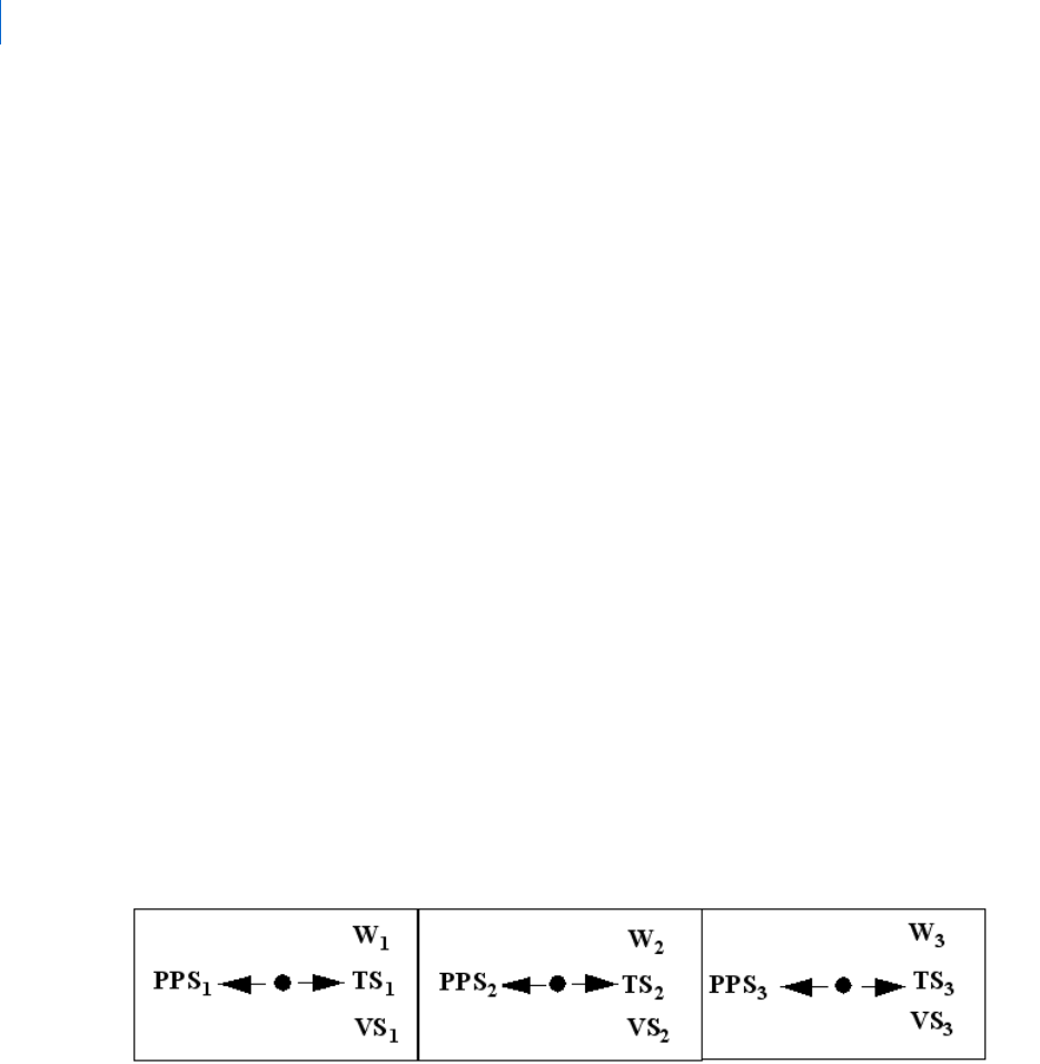
Gas Dynamics Library User Guide

Introduction

This section discusses the components in the Pipes and Flow Resistances group of the Gas Dynamics Library.

This group includes

 The discretizable PC lumped parameter transient-momentum pipe

 The discretizable PX Method of Characteristics (piecewise continuous) pipe

 The resistive component PR (pipe or annulus)

 The FL and FR Flow Resistance components. These components are non-discretizable, and use flow

models based upon K-factors or vs. flow, where is the specific gravity

Lumped parameter pipe and flow resistance models are also important in modeling components in the Heat

Exchangers, Minor Losses and Boundary Components groups:

 The HS and HT heat exchanger components are adaptations of the PC pipe

 Other heat exchangers use flow models similar to FL and FR

 All components in the Minor Loss group, as well as certain Boundary Components, are derived from

component FL

The Method of Characteristics is the most efficient way to model fluid transients where wave or acoustic

effects may be important, but is limited to single-phase gas flow and often yields a less accurate steady-state

mass balance. The Method of Characteristics also seems to work better for situations where the density or

volume are small. The lumped parameter method gives the most accurate steady-state mass balance, and is

the only method in the Gas Dynamics library that presently handles 2-phase flow.

Discretization of PC and PX

Both PC and PX are discretizable, but there are differences in how they are discretized. Consider a pipe with

three sections. Each section of the PC pipe is considered a lumped parameter, meaning that each section is

considered to have a uniform temperature, pressure and velocity (the arrows indicate data flow):

The PX pipe is piecewise continuous, so the discretization of a pipe with three sections results in four mesh

points:

σΔp

Main Index

Chapter 6: Pipes and Flow Resistances

Fundamental Equations- Lumped Parameter, Transient Momentum

The PX pipe always contains one more mesh point than sections, and the minimum dimension for J, the

number of mesh points or nodes, is 2.

Fundamental Equations- Lumped Parameter, Transient

Momentum

Equations of Continuity

In this section the mathematical model for the PC (Discretized Lumped Parameter Pipe) and PR (Resistive

Pipe or Annulus) is presented. Material balance equations for a pipe volume are the same as for any other

volume, and are given in Chapter 4: Nodes and Volumes. All pipe volumes are considered constant-

compliance is not modeled. The discretized continuity equation species n, at finite difference node j, where

the total number of species is the component dimension I, is

where P

s,i

[state PPS(i)] is the partial pressure of species i (equal to the static pressure for I=1)

and is P

the species density (equal to the static fluid density for I=1).

The partial derivatives are evaluated with the subscripted quantities (outside of the parentheses) held

constant.

If j=1

then w

2,n,j-1

is replaced by w

1,n

Condensation Rate

The components in the Pipes group always use the mass transfer model except when H

O is the only fluid

species. In this case the bulk condensation model is used. Details of these models are given in Chapter 4.

xΔ p

sij,,

∂

--------





1 kj,,

, ki≠,

i 1=



Sj,

∂

T∂

--------















2 nj 1–,,

2 nj,,

–=

(6-1)

Main Index

Gas Dynamics Library User Guide

Fundamental Equations- Lumped Parameter, Transient Momentum

Equation of Energy

The total energy balance is

The term

is simply equal to -1 for an ideal or perfect gas.

The discretized energy equation is,

represents the fluid enthalpy, the fluid density, and c

the fluid specific heat. The flow rates in the

preceding equations are:

The quantity p

1,j

is the static pressure at node j, which is the sum of the species partial pressures p

1,j,i

, and

is the sum of the species densities

i,j

. Additionally:

The quantity w

2,j

is the sum of w

2,n,j

. Fs is given by Equation (6-3).

Heat Transfer Calculation

All heat transfer correlations in this section can be found in Reference 1. The heat transfer from the pipe wall

to the gas is calculated as

V ρc

----------

–





---

ρ∂

T∂

------











h–()q

– w

++=

(6-2)

---

ρ∂

T∂

------





xΔρ

Pj,

Sj,

---------

ρ∂

T∂

------





1 j,





2 j,

M()

j 1–

–()W

2 j,

m()

j 1+

–()–[]Q

IN j,

sj,

–+=

(6-3)

2 j,

M()

max w

2 j,

0,()= w

2 j,

m()

min w

2 j,

0,[]=

Sj,

,(),= h

S 1,

,(),= h

J 1+

,()=

Pj,

Sj,

()= ρ

ρ p

Sj,

,()=

2⁄=

IN j,

πD

xΔ T

Wj,

Sj,

–()=

(6-4)

Main Index

Chapter 6: Pipes and Flow Resistances

Fundamental Equations- Lumped Parameter, Transient Momentum

The input parameter HTC is used for the heat transfer coefficient if it is not less than zero. If HTC is less

than zero, the heat transfer coefficient is given by , where the laminar flow/natural

convection Nusselt number is

or the turbulent flow Nusselt number is:

and

κ is the thermal conductivity. The Prandtl number Pr is given by:

and the Graetz number is RePrD

/L. The subscript f denotes evaluation of fluid properties at the film

temperature T

=0.5(T

), and the Graetz number is based upon total pipe length L and not upon x.

The wall temperature rate is

Equation of Momentum

In the equations that follow, a lower-case j indicates the finite-difference index, and the upper-case J is the

component dimension J, the total number of finite-difference control volumes.

Molecular, Mixed Molecular/Viscous, and Viscous Flow (ZSW=0,1, or 2)- A linear velocity/shear force

relation is assumed:

where Rflow is the flow resistance. For molecular flow (ZSW=0):

Nu κ D

⁄()=

Nu 3.66

0.19Gz

0.8

1 0.117Gz

0.467

----------------------------------------

----





0.14

(6-5)

Nu 0.023Re

0.8

0.4

(6-6)

μc

--------

W9 j,

4 Q

+()

xΔπD

–()c

pW,

-------------------------------------------------------

(6-7)

flow

sj,

πD

-----------

–=

(6-8)

flow

sj,

xΔ

------------------

(6-9)

Main Index

Gas Dynamics Library User Guide

Fundamental Equations- Lumped Parameter, Transient Momentum

where p

is the static pressure, and v

is the molecular velocity, given by (2):

For laminar flow (ZSW=2):

For mixed laminar/molecular flow (ZSW=1):

Turbulent, Non-choked Flow (ZSW= 3)- The friction factor for turbulent flow (3) is given by:

where the Reynolds number Re is given by

The shear force is:

Discretized Transient Momentum Balance- The momentum balance, for 1<j<J, is:

if j=1:

8RT

------------=

(6-10)

flow

32μ xΔ

----------------

(6-11)

flow

1–

xΔ

---------------





1–

32μ xΔ

----------------







1–

(6-12)

′±

0.0791 Re

0.25

⁄ Re 4000>,

0.008 9.7314

7–

×10 Re 2000–()– 2000 Re 4000≤≤,







(6-13)

sj,

------------------------

(6-14)

sj,

sign

---

fρ

sj,

πD

-----------

,()–=

(6-15)

xΔ u

sj,

dvs

Main Index

Chapter 6: Pipes and Flow Resistances

Fundamental Equations- Lumped Parameter, Transient Momentum

where

and if j=J:

Choked flow (ZSW=4)- The velocity constraint is

where c

is the sonic velocity:

In this case, the velocity equation is a constraint without time derivatives. However, the velocity derivatives

continue to appear in the energy equation.

During choked flow the momentum balance quantity dvs

is also calculated from the non-choked formula

in the previous paragraph for use in switch-state logic.

Frequency-Dependent Shear Force Terms- The frequency dependent shear force terms are given by:

2 j 1–,

sj 1–,

sj,

–()F

sj,

sj 1+,

–()A

1 j,

2 j,

3 j,

++()++ +=

(6-16)

xΔ u

sj,

dvs

sj,

–()F

sj,

sj 1+,

–()A

1 j,

2 j,

3 j,

++()++ +=

(6-17)

ρ pp

,()A

------------------------------------

0>,

--------------

0≤,







(6-18)

xΔ u

sj,

dvs

2 j 1–,

sj 1–,

sj,

–()F

sj,

–()A

1 j,

2 j,

3 j,

++()++ +=

(6-19)

sj,

sign c

sj,

sj 1–,

–,()=

(6-20)

ρ∂

P∂

------





-----

ρ∂

T∂

------





–

-----------------------------------------------

(6-21)

ij,

sj,

sj 1+,

–()α

⁄ XX

ij,

+= XX

ij,

μY

ij,

ρr

⁄–=

(6-22)

Main Index

Gas Dynamics Library User Guide

Fundamental Equations- Lumped Parameter, Transient Momentum

where r

/2 and the

are the roots of the equation , J

(

) = 0, J

is the Bessel function of the first kind

of order zero. The first three values of

are 2.4048, 5.5201 and 8.6537.

Two-phase flow (4)- When moisture condensate is present, indicated by SWC=1, then the effective mixture

viscosity is calculated from the McAdams equation:

and the effective mixture density is calculated as:

where x is the quality (mass fraction gas).

Switch State Rate Calculation

The switch state SMC indicates whether a single phase gas or two phase mixture (gas + H

(l)

) is present.

This switch state is active only if 1) H

O is one of the fluid species and 2) the GP component parameter WX

is set to one. An SMC value of zero indicates a single gas phase, a value of one indicates gas+liquid, and a

value of two indicates single phase liquid (possible if and only if H

O is the only fluid species).

Mass transfer model- The rate of the switch state SMC is given by

If none of these conditions is satisfied then dSMC = SMC.

Bulk condensation model- The rate of the switch state SMC is given by

where is the void fraction (V

/V). If none of these conditions is satisfied then dSMC = SMC. SMC or dSMC

can be equal to 2 if and only if H

O is the only fluid species.

-----

1 x–

-----------





1–

-----

1 x–

-----------





1–

dSMC

1 , if SMC 0= and w

lin,

lex,

+–0>

0 , if SMC 1= and w

lin,

lex,

+–0< and m

0≤







dSMC

0 , if SMC 1= and w

lin,

lex,

+–0< and m

0≤

1 , if SMC 0= and p

sat

()>

1 , if SMC 2= and p

sat

()<

2 , if SMC 1= and p

sat

()> and ϕ 0=











Main Index

Chapter 6: Pipes and Flow Resistances

Method of Characteristics

The Method of Characteristics transforms the partial differential equations of continuity (L

), energy (L

)

and momentum (L

into three ordinary differential equations each defined along a characteristic curve :

where A is the cross-sectional area, q is the heat transfer or generation per unit volume, fs is the shear force

per unit volume, c is the sonic velocity and

At each interior node (mesh point) the three characteristic equations are solved for the local pressure,

temperature and velocity. Only the forward characteristic (dx/dt = v - c) is applicable at the inlet (J=1), and

only the backward characteristic (dx/dt = v + c) is applicable at the exit (J = # of nodes). The applicable

boundary characteristics are used to solve the boundary pressures.

The inlet port of the Method of Characteristics pipe (PX) can be configured as storage (flow input, pressure

output) or resistive (pressure input, flow output), and the same is true of the exit port. The storage port is the

ρ∂

t∂

------

ρv∂

x∂

---------

ρv

------

A∂

x∂

------

++==

(6-23)

---

ρ∂

T∂

------





P∂

t∂

------

P∂

x∂

------

+ ρc

T∂

t∂

------

T∂

x∂

------

+ qvf

–()–+==

(6-24)

0 ρ

v∂

t∂

-----

ρv

v∂

x∂

-----

P∂

x∂

------

–++==

(6-25)

------

---

------

-----

-------

+ R

---

------

vc+=,

(6-26)

---

–

------

-----

-------

+ R

---

–=

------

vc–=,

(6-27)

---

ρ∂

T∂

------





------

ρc

------

+ qvf

–=

-----

v=,

(6-28)

ρ∂

T∂

------





qvf

–()

ρc

--------------------

–

ρv

------

A∂

x∂

------

–=

Main Index

Gas Dynamics Library User Guide

Flow Resistances and the Minor Loss group

simplest. When a port is configured as resistive an orifice model and discharge coefficient is added. For

example, a resistive PX inlet is equivalent to a storage PX inlet connected to an OR orifice with the same

diameter as the pipe.

Component PX is recommended when accurate modeling of transients in a single-phase gas is needed.

Experience so far has indicated that this component also works better than PC if the density or volume

become small. The weaknesses of PX are that 1) the steady-state mass balance is less accurate and 2) it is

limited to a single phase.

The default configuration for component PX employs a modified Method of Characteristics that results in a

more accurate steady-state mass balance. An alternate configuration with a "classical" Method of

Characteristics is also available. At zero steady velocity the modified Method of Characteristics is equivalent

to the “classical” Method of Characteristics.

Flow Resistances and the Minor Loss group

The simplest flow resistance component is FL in the default Resistive configuration. FL can also be

configured as Storage/Resistive, which is equivalent to Resistive FL connected to an upstream node NO. A

number of resistance formulations are available:

 tabulated flow vs. p, where is the specific gravity. (The reference density for specific gravity is

a global input to component GP).

 analytical flow vs. p, where p= Zw

, where the default value of a = 2.

 constant K-factor,

 K-factor as a tabulated function of Reynold number

 K-factor as a tabulated function of 1, 2 or 3 connected inputs

 K-factor as a tabulated function of Reynolds number and 1 or 2 connected inputs

The components in the Minor Losses groups are derived from one of the FL tabular K-factor configurations,

with default tabular data. Most of these are available as Resistive or Storage/Resistive. The default tabular data

is taken from Reference 5.

Component FR is a Storage/Resistive flow resistance. It is designed to model flow resistance with multiple

heat loads, such as an air-cooled equipment rack on an aircraft. Provision is made for both conduction

(including convection) and radiation heat transfer between the heat loads, from each heat load to the gas,

from each heat load to the wall or enclosure, and from the enclosure to ambient. FR also comes with a “zero-

resistance feed-through” configuration, which does not have a pressure state, and which should be used if flow

resistance is negligible but heat transfer needs to be modeled.

Guidelines for Component Selection and Use

Use either the PC or PX components when the detailed geometry of a pipe is known, and a detailed pressure

profile is needed. The PC component can be used for single phase gas flow or two phase applications. It is

most accurate for steady-state calculations. When moisture condensation is present it is recommended that

σΔ

ΔpK

ρv

--------

Main Index

Chapter 6: Pipes and Flow Resistances

References

consideration of transient shear be disabled by setting FDS=0. The PI, PV and PW components are now

obsolete. PX is the most accurate for transient analyses, and is also the most robust when the density or

volume is very low.

A pipe component with a very low resistance, such as a short, large diameter pipe, can cause a simulation to

become very slow or to fail, particularly when the pipe is PC. This happens because the calculated flow or

velocity becomes extremely sensitive to the pressure difference, causing numerical difficulties for the

integrator, and can be diagnosed by selecting “Print Detailed Diagnostics” in the Analysis Data Form. The

best solution to this problem is usually to lump the pipe volume with the volume of an adjacent component.

Component PR is recommended when 1) a resistive pipe is needed, 2) PC or PX are causing marked increases

in simulation CPU times or 3) annular geometries need to be modeled. Since this pipe is a pure resistance,

no pressure or velocity states are added to the model when this component is used.

Use the FL or FR component to model a more generalized flow resistance, such as a resistance that is

correlated by sigma* P vs. flow. FL is the simpler of the two components, particularly in the default resistive

configuration. The FR component is used when it is necessary to model internal heat transfer for a flow

resistance with multiple heat sources. Both FL and FR are steady-momentum components.

The Minor Loss group of components is primarily intended for use in steady-state modeling. Since the losses

are small and the volumes are usually also small, transient simulations with these components often results in

very large CPU times, when compared with the same model without the Minor Loss components.

References

1. J.P. Holman, Heat Transfer, 4th Ed., McGraw-Hill, New York (1976).

2. S. Dushman and J.M. Lafferty, Scientific Foundations of Vacuum Technique, 2nd Ed., Wiley, New

York (1962).

3. N. DeNevers, Fluid Mechanics, Addison Wesley, Reading, MA (1977).

4. J.G. Collier and J.R. Thome, Convective Boiling and Condensation, Oxford (1994).

5. Thermodynamics of Incompressible and Compressible Fluid Flow, SAE AIR1168/1 (2004).

Main Index

Gas Dynamics Library User Guide

References

Main Index

Chapter 7: Heat Exchangers

MSC Nastran Implicit Nonlinear (SOL 600) User’s GuideGas Dynamics Library User Guide

Heat Exchangers



Introduction 78



Heat Exchangers- Single Pressure State, Discretized Temperature Array 81



Heat Transfer Coefficient Calculation (Components HE, HF, HS and HT) 83



Heat Exchanger Flow Calculation 83



Switch State Rate Calculation 84



Guidelines for Component Selection and Use 85



Bibliography 85

Main Index

Gas Dynamics Library User Guide

Introduction

The Heat Exchangers groups contains three different sets of components:

 Heat exchangers based upon efficiency maps (HK, HL),

 Heat exchangers based upon heat transfer coefficients with a single pressure state and discretized

temperature states (HE, HF) and

 Heat exchangers based upon heat transfer coefficients with discretized pressure and temperature

states (HS, HT).

The HK and HL components each represent complete heat exchangers, while the other Gas

Dynamic Library Heat Exchanger components model only a portion of the heat exchanger and are normally

discretized.

Two components, a primary component and a secondary component connected through Port 9, are required

to model a heat exchanger unless HK or HL are used.

HF and HT are primary components, which model a fluid and the heat exchanger core, calculating the rate

of the core temperature state. HE and HS are secondary components that model heat transfer from the

secondary fluid to the heat exchanger core.

Figure 1 illustrates the connection between primary and secondary heat exchanger components.

Figure 1 Heat Exchanger Components Connection

Heat Exchangers Based on Effectiveness Maps

Gas/Gas Heat Exchanger

The HK component models a gas/gas heat exchanger based upon effectiveness maps. This component is

equivalent to two thermally connected volume components as shown in Figure 2.

Main Index

Chapter 7: Heat Exchangers

Heat Exchangers Based on Effectiveness Maps

Figure 2 Two Thermally Connected Volume Components

Refer to Chapter 4: Nodes and Volumes for the detailed model of the volumes.

The steady-state heat transfer between the hot-side volume (flow between Port 1 and Port 2) and the cold-

side volume (flow between Port 3 and Port 4) is

where is the heat exchanger effectiveness and

The transient heat flow is modeled as

The designation of hot-side and cold-side is arbitrary, and establishes the sign convention for Q

. A negative

value of Q

w,ss

means that the fluid entering the Port 3-Port 4 volume is actually warmer than the fluid entering

the Port 1-Port 2 volume.

The bulk condensation model (Chapter 4) is used to model phase change in the HK component, since the

wall temperature is not calculated or known.

If transient analysis is anticipated, then please make sure to read the section below titles “

Limitations of Transient

Analysis Using Effectiveness Models

”

wss,

ηC

min

hin,

cin,

–()=

(7-1)

min

min w

p 2,

p 4,

,()=

(7-2)

wss,

–

---------------------------

(7-3)

Main Index

Gas Dynamics Library User Guide

Heat Exchangers Based on Effectiveness Maps

Gas/Liquid Heat Exchanger

The gas/liquid heat exchanger HL is similar to the HK component, except that the cold side is modeled as a

liquid with constant specific heat. The liquid flow, pressure and pressure rate are simply passed through ports

3 and 4:

Hence, the liquid flow calculations must be done by a component connected to port 3 of HL, or else the

liquid flow W3 must be set as a constant parameter. Ports 3 and 4 are configured to make default ported

connections with the Easy5 Thermal Hydraulics (hc) library as a storage-resistive component.

Limitations of Transient Analysis Using Effectiveness Models

The definition of heat exchanger effectiveness is based upon a steady-state model, and there are risks

associated with the application of this concept to transient problems: if a physically realistic time constant is

used with component HK or HL, then transient violations of the 2nd Law of Thermodynamics may occur.

The remedy, if this occurs, is to reduce the time constant so that the heat exchanger is always closer to steady

state. The default value for the time constant in components HK and HL is 0.01, which is much smaller than

what would be considered physically realistic, but which seems to keep transient 2nd Law violations from

occurring.

One option for slowing the transient response that use effectiveness maps and the small default value of the

time constant is to use additional HF component(s), not connected to secondary heat exchange

component(s), to model the thermal mass of the heat exchanger core:

Main Index

Chapter 7: Heat Exchangers

Heat Exchangers- Single Pressure State, Discretized Temperature Array

Figure 3 Using HF Component to Slow Transient Response

The equations that define effectiveness are based upon the assumption of constant specific heat. But unless a

perfect gas is specified, specific heat is a function of temperature in the Gas Dynamics library. So hand

calculations of heat transfer may not exactly agree with the heat transfer calculated by an Easy5 model.

Heat Exchangers- Single Pressure State, Discretized

Temperature Array

The HF (primary fluid + core) and HE (secondary fluid) components can be used together to model parallel

flow, counterflow and crossflow heat exchangers with the gas and core temperatures discretized in two

dimensions (modes J and K). These components can also be thermally connected through the “wall” port to

heat exchanger components in the HC, VC and EC libraries.

Equations of Continuity

The transient material balance considers only the pressure rate. The discretized continuity equation species

n, at finite difference node j, where the total number of species is the component dimension I, is

where P

s,i

[state PPS(i)] is the partial pressure of species i (equal to the static pressure for I=1) and

is the

species density (equal to the static fluid density for I=1). The partial derivatives are evaluated with the

subscripted quantities (outside of the parentheses) held constant.

∂

--------





i 1=













1 n,

2 n,

–=

(7-4)

Main Index

Gas Dynamics Library User Guide

Heat Exchangers- Discretized Pressure and Temperature Vector

Condensation Rate

The mass transfer model is employed except when H

O is the only fluid species, in which case the bulk

condensation model is used. Details of these models are given in Chapter 4. The condensation calculation is

discretized.

Equation of Energy

The transient energy equation considers only the discretized temperature arrays. The discretized fluid energy

balance is

and the discretized core energy balance (modeled by the primary component) is

Transient Response

The left-hand-sides of continuity (7-48) and energy (7-49) differ from more rigorous equations in Chapter

4: the term is missing from equation 7-48, while the is missing from equation 7-49. The equations are

formulated this way because, in general, there are a different number of temperature and pressure states-

temperature is a discretized array while pressure is considered uniform throughout the fluid volume.

Therefore, the model will give the correct steady-state results but transient results may deviate from what

might be expected from a rigorous transient model

Heat Exchangers- Discretized Pressure and

Temperature Vector

The HT (primary fluid + core) and HS (secondary fluid) components can be used together to model parallel

flow, counterflow and crossflow heat exchangers with the gas and core temperatures discretized in a single

dimension (mode J). These components can also be thermally connected through the “wall” port to heat

exchanger components in the HC, VC and EC libraries.

The mathematical model for the HT and HS component is equivalent to one or more parallel steady

momentum pipes (PI), and is described in Chapter 6. The parameters LWF (flow length), AXF (average flow

cross-sectional area) and AHT (heat transfer area) are used to determine the appropriate scale factor, the

number of parallel flow paths.

Vρc

{}

jk,

hp T

jk,

,()–[]q

wjk,,

cjk,,

++ +=

(7-5)

JK×

-------------

wjk,,

–=

(7-6)

Main Index

Chapter 7: Heat Exchangers

Heat Transfer Coefficient Calculation (Components HE, HF, HS and HT)

Heat Transfer Coefficient Calculation (Components HE,

HF, HS and HT)

The modeler can choose between entering a constant value for the heat transfer coefficient, calculating the

heat transfer coefficient in a User-code block and connecting to the heat transfer coefficient input, or

calculation of the heat transfer coefficient by the heat exchanger component. If the latter option is chosen

then the heat transfer correlations for circular pipes, given in Chapter 6: Pipes and Flow Resistances of this

guide, are used. The input parameter DH (hydraulic diamter) is used as the diameter in the heat transfer

coefficient correlations, while the pipe length used in the correlation is LWF.

Heat Exchanger Flow Calculation

Tabular Correlation

The option to use a tabular flow correlation is available for heat exchanger components that have a single

pressure state- the HE, HF, HK and HL (gas side only) components. The form of the correlation is

vs. flow, where is the specific gravity. The value of the reference density is specified in the GP component.

This option is not available for the HS or HT components, since calculation of a discretized pressure profile

requires a more detailed specification of the component geometry.

Analytical Correlation

The option to use an analytical flow correlation is available for heat exchanger components that have a single

pressure state- the HE, HF, HK and HL (gas side only) components. The form of the correlation is

p = Zw

where is the specific gravity and a has a default value of 2. The value of the reference density is specified

in the GP component.

This option is not available for the HS or HT components, since calculation of a discretized pressure profile

requires a more detailed specification of the component geometry.

Steady-momentum pipe model (equivalent pipe)

This method is available for heat exchanger components that have a single pressure state- the HE, HF, HK

and HL (gas side only) components. The parameters LWF (flow length) and AXF (average flow cross-

sectional area) are used to model the component as a set of parallel pipes using the same equations as are

presented in Chapter 7 for a steady-momentum pipe.

Zero-resistance flow-through

This method is available for the HE, HF, HK and HL components, and is always used for the liquid side of

HL. The flow and pressure rate are not calculated by the heat exchanger component- flow and pressure are

σΔp×

σΔ

Main Index

Gas Dynamics Library User Guide

Switch State Rate Calculation

inputs to the component and are passed through: w

exit,i

= w

inlet,i

and pp

inlet,i

= p

pexit,i

. Although this

configuration has a Storage/Resistive architecture, pressure (pp

inlet,i

) is not a state but an algebraic variable.

The fluid and core temperature arrays are dynamic states in this configuration, just as they are in the other

heat exchanger configurations.

A heat exchanger component with a pressure-state and a very small flow resistance may challenge a variable-

step integrator and result in long execution times. Using the zero-resistance flow-through configuration in

such cases may result in greatly improved execution times.

Transient-momentum pipe model (equivalent pipe)

This method is available for heat exchanger components that have a discretized pressure state- the HS and

HT components. The parameters LWF (flow length) and AXF (average flow cross-sectional area) are used to

model the component as a set of parallel pipes using the same equations as are presented in Chapter 7 for a

transient-momentum pipe.

Switch State Rate Calculation

The HE, HF, HL, HS and HT components each have a switch state named SMC that indicates either a single

phase or two phase mixture. The HK component has two of these switch states, SM1 and SM3. This switch

state is active only if 1) H

O is one of the fluid species and 2) the GP component parameter WX is set to

one. An SMC value of zero indicates a single gas phase, a value of one indicates gas+liquid, and a value of two

indicates single phase liquid (possible if and only if H

O is the only fluid species).

Mass transfer model (HE, HF, HS and HT)- The rate of the switch state SMC is given by

If none of these conditions is satisfied then dSMC = SMC.

Bulk condensation model (HK and HL)- The rate of the switch state SMC is given by

where is the void fraction (V

/V). If none of these conditions is satisfied then dSMC = SMC. SMC or dSMC

can be equal to 2 if and only if H

O is the only fluid species.

dSMC

1 , if SMC 0= and w

lin,

lex,

+–0>

0 , if SMC 1= and w

lin,

lex,

+–0< and m

0≤







dSMC

0 , if SMC 1= and w

lin,

lex,

+–0< and m

0≤

1 , if SMC 0= and p

sat

()>

1 , if SMC 2= and p

sat

()<

2 , if SMC 1= and p

sat

()> and ϕ 0=











Main Index

Chapter 7: Heat Exchangers

Guidelines for Component Selection and Use

The selection of heat exchanger components will be constrained by the type of experimental data that is

available:

1. If the data is in the form of efficiency maps, use the HK or HL components.

2. If the heat transfer coefficients for each fluid and the core thermal mass are known then:

• If a tabulated flow correlation is needed, use HE and HF.

• If good estimates are available for AXF, LWF and AHT, use HE/HF or HS/HT.

The discretized pressure profile of HS and HT enables a more rigorous formulation than is possible for a

single pressure state, and is especially preferable for high velocity gas flow. However, the HE and HF

components have the advantage of being discretizable in two dimensions, while the HS and HT components

may only be discretized in a single dimension.

Bibliography

1. J.P. Holman, Heat Transfer, 4th Ed., McGraw-Hill, New York (1976).

Main Index

Gas Dynamics Library User Guide

Bibliography

Main Index

Chapter 8: Chemical Reactors

MSC Nastran Implicit Nonlinear (SOL 600) User’s GuideGas Dynamics Library User Guide

Chemical Reactors



Introduction 88



Mathematical Model 88



Guidelines for Component Selection and Use 92



Bibliography 92

Main Index

Gas Dynamics Library User Guide

Introduction

The Chemical Reactors group consists of two components that each model a single chemical reaction, ER

and CR. ER calculates the equilibrium extent of reaction and CR requires the user to input the extent of

reaction. Both components calculate the adiabatic chemical reaction temperature. Future releases of the Gas

Dynamics Library will contain a component for calculating equilibrium extents of reaction for multiple

chemical reactions, and also contain components for modeling chemical kinetics.

The CR and ER components are designed to be connected to an inlet port of node such as NO. The total

pressure in the CR or ER component is equal to the static pressure in the volume component to which it is

connected. The CR and ER component each contain an implicit constraint state, the adiabatic reaction

temperature TF_Exit, so the RADAU54 integrator must be used for transient analysis of models containing

these components.

Mathematical Model

Stoichiometric Coefficients

A general, but somewhat abstract way of specifying a chemical reaction is through the use of a stoichiometric

coefficient vector :

where M

represents the chemical symbol for the species.

The species, and their places in the stoichiometric coefficient vector, are specified by the GAS (vector)

parameter in the GP component (if MUI=1) or GM component (MUI=2,3,4,or 5).

Example: Methane combustion in pure oxygen- This reaction is

which can be written as

The stoichiometric coefficients are:

 CH

: -1

 O

: -2

 CO

: 1

 H

O: 2



(8-1)

+ CO

O+=

1CH

–2O

1CO

O++–0=

Main Index

Chapter 8: Chemical Reactors

Mathematical Model

If the GP component GAS vector parameter were specified as:

 GAS(1) = 10 (CH

)

 GAS(2) = 3 (O

)

 GAS(3) = 6 (CO

)

 GAS(4) = 4 (H

then

 = -1

 = -2

 = 1

 = 2

Example 2: Methane combustion in air- This is the same reaction as Example 1, but an additional inert species

) is now present. The stoichiometric coefficient of an inert species is zero, since does not appear in the

chemical equation. If the GP component GAS vector parameter were specified as:

 GAS(1) = 10 (CH

)

 GAS(2) = 3 (O

)

 GAS(3) = 6 (CO

)

 GAS(4) = 4 (H

 GAS(5) = 2 (N

)

then

 = -1

 = -2

 = 1

 = 2

 = 0

Be sure to specify a stoichiometric coefficient for each fluid species, even if it is inert.

Main Index

Gas Dynamics Library User Guide

Mathematical Model

Extent of Reaction

The extent of reaction can be defined in terms of any of the non-inert species as

where n

is the exit molar flow n and is the inlet molar flow of species i. The exit flow of all species can be

specified in terms of the extent of reaction:

The limiting extent of reaction is:

The reactant (negative stoichiometric coefficient) species for which

is a minimum is called the

limiting reactant, and all other reactants are present in excess. The CR component calculates the extent of

reaction as , where F

is an input parameter supplied by the user. The ER component

calculates the thermodynamic equilibrium extent of reaction.

Equilibrium Extent of Reaction

The criteria for chemical equilibrium for a single chemical reaction is

where K is the equilibrium constant, calculated in terms of the species Gibbs free energies of formation G

f,i

and the temperature state in the downstream volume component:

–

----------------

(8-2)

ε+=

(8-3)

lim

min

–

--------

–

--------

–

--------

…,,,()=

evaluated for all reactants.

– ν

⁄

εε

lim

Kln ν

()ln



(8-4)

Kln

fi,



RTR

exit

⋅

-----------------------

–=

(8-5)

Main Index

Chapter 8: Chemical Reactors

Mathematical Model

Since

where

the chemical equilibrium equation, in terms of the extent of reaction, is

This equation is numerically solved at each model call for the extent of reaction , and the exit flows then

calculated as

where M

is now the molecular weight.

If then the flow through the reactor is equimolar, and static pressure in the reactor (calculated by the

downstream volume component) has no influence on the extent of reaction.

≠ 0 then the exit total molar flow will be a function of the extent of reaction, and pressure rate in the

downstream volume will be coupled with the extend of reaction.

Adiabatic Reaction Temperature

The adiabatic reaction temperature TF

EXIT

is also called the adiabatic flame temperature when the reaction

is a combustion reaction, and is calculated by considering the reactor as isenthalpic. The following

thermodynamic path is used:

The enthalpy difference between thermodynamic states (2) and (3), in terms of the species enthalpies of

formation H

f,i

----

ε+

νε+

-------------------

p===

(8-6)

νν



and

Kln ν

ε+()ln



ν n

νε+()ln ν p()ln+–=

(8-7)

2 i,

1 i,

ε+ M

(8-8)

ν 0=

(1) Reactants at TF

inlet

(2) Reactants at TF

exit

(3) Products at T

exit

– εν

fi,



(8-9)

Main Index

Gas Dynamics Library User Guide

Guidelines for Component Selection and Use

and the implicit constraint equation for T

The adiabatic flame temperature is formulated as an implicit constraint state, and models that contain a CR

or ER component must use the RADAU54 integrator. The Implicit formulation configuration should be

used by all components in a model that contains CR or ER.

Non-adiabatic Reactor Modeling

Heat transfer to/from the reactor can be modeled in the downstream node or volume component, and the

resulting temperature is passed to the reactor component as TR

exit

, which is the temperature used in the

chemical equilibrium calculation.

Guidelines for Component Selection and Use

 Use CR if chemical equilibrium is not attained, and input the fractional conversion F

 Use ER to model reactions that attain chemical equilibrium.

 Always connect CR or ER to a downstream volume component (NO, ND, N2, VX or VY)

 Use the RADAU54 integrator for simulations of models containing CR or ER components.

Bibliography

1. J.M. Smith and H.C. Van Ness, Introduction to Chemical Engineering Thermodynamics, 4th Ed.,

McGraw-Hill, New York (1987).

2. K.G. Denbigh, The Principles of Chemical Equilibrium, 3rd Ed., Cambridge (1977).

εν

fi,



Hp T

,()Hp T

,()–+0=

(8-10)

Main Index

Chapter 9: Compressors, Fans, & Turbines

MSC Nastran Implicit Nonlinear (SOL 600) User’s GuideGas Dynamics Library User Guide

Compressors, Fans, &

Turbines



Introduction 94



Compressors 94



Fan 98



Turbine 98

Main Index

Gas Dynamics Library User Guide

Introduction

The Compressors, Fans and Turbines group contains two compressor components, one fan and one turbine

component. Unlike most other components in the Gas Dynamics library, these components are not designed

to handle reverse flow.

Compressors

Compressor Based upon Corrected Flow Map (CN)

Figure 1 shows a typical performance map for a conventional centrifugal compressor. The map plots pressure

ratio (P

) as a functions of corrected mass flow and corrected speed . P

, T

, and w1

are inlet conditions to the compressor or fan, P

is the outlet pressure, and N is the rotational speed. The

performance map also shows lines of constant efficiency.

Component CN uses a third intermediate parameter called the grid parameter or iteration parameter. The

lines labeled “Grid lines” in

Figure 1 are rays that originate from a arbitrary common point outside of the

performance map. Each line is assigned a value which is the grid parameter. The assigned values are somewhat

arbitrary, but they must be monotonically increasing or decreasing. Since the grid parameter is an

independent variable in a table lookup it is also advantageous if the values are equally spaced.

Component CN uses three tables:

GR: Grid parameter as a function of pressure ratio P

and corrected speed

WC: Corrected flow as a function of P

and

ET: Efficiency as a function of P

and

()P

⁄

⁄()

()P

⁄

⁄()

Main Index

Chapter 9: Compressors, Fans, & Turbines

Compressors

Figure 1 Compressor Map

Main Index

Gas Dynamics Library User Guide

Compressors

The temperature increase in the compressor is

where

γ is the specific heat ratio C

if the gas is ideal, or if the gas is not ideal

where Z is the compressibility factor, assumed constant and evaluated at the inlet conditions.

The species pressures at the inlet port are calculated as

and the inlet port static pressure rate is given by

The compressor work is given by

which (like the compressor maps) is rigorous only at steady state.

Compressor Based upon Map of Polytropic Efficiency and Polytropic Head

(CP)

Component CP, in the Polytropic configuration, models a gas compressor based upon tabular inputs for

polytropic efficiency and polytropic head as functions of compressor speed and volumetric suction flow. It is

designed to be used in conjunction with upstream and downstream volumes that model the compressor inlet

and exit chambers. The inlet chamber can be modeled by an NO component (Storage/Resistive architecture),

and the exit chamber can be modeled by NO (any architecture). The downstream chamber could also be

modeled by the volume (parameter V1) associated with a storage/resistive OR component, which can also

model an exit orifice.

This compressor component, unlike most other components in the GD library, does not model reverse flow.

However, the reverse flow inputs and outputs, (TR, KR and Q) are included in order to enable default ported

connections to other GD library components

Performance Equations- The polytropic efficiency relates the compressor performance to the isentropic

performance through the relation:

–

---------

------





γ 1–

------------

1–=

ZR–

--------------------

i() P

i()



---------------------

ZRT

–

-------------------

WKC H T

,()HT

,()–=

n 1–

------------

pol

κ 1–

------------

Main Index

Chapter 9: Compressors, Fans, & Turbines

Compressors

where n is the polytropic coefficient and k is the specific heat ratio C

calculated at the inlet conditions.

The ratio is calculated as

which reduces to for an ideal gas. The constraint equation governing the suction side

pressure is:

where the polytropic head is the result of the input table HPL and

where the subscript s denotes suction side conditions, Z

is the compressibility, g is the gravitational

acceleration, and P

is the static downstream pressure, given by

The upstream species pressures are given by:

The absolute exit temperature is given by:

where is the absolute suction temperature. The volumetric suction flow is given by

and the power consumption is given by

κκ1–()⁄

κ 1–()

-----------------

ρ∂

P∂

------





ρ∂

T∂

------





----------------------------

κκ1–()⁄ C

R⁄=

() 0 H

pol table,

pol calc,

–==

pol table,

pol calc,

---------------

n 1–

------------

------





n 1–

------------

1–=

2 j,

j 1=



1 j,

2 j,

------------

------





n 1–

------------

1 j,



ρ P

,()

-------------------------

Main Index

Gas Dynamics Library User Guide

Fan

Component FM uses two tables:

FLW: Volumetric flow as a function of P

-P

or (P

-P

)/σ, where σ is the specific gravity.

ET: Efficiency as a function volumetric flow.

The independent variables of Easy5 tables are required to be monotonic, but P

-P

may not be monotonic.

An alternate configuration of component FM is available in this case, in which the first table has P

-P

)/σ as a function of volumetric flow. This disadvantage of this alternate configuration is that there will

be an additional flow constraint state that must be initialized. RADAU54 must be used for simulations of

models containing this alternate configuration.

The exit temperature TF_Exit is calculated as

where

γ (the ratio of specific heats if the gas is considered ideal) is

The species pressures at the inlet port are calculated as

and the inlet port static pressure rate is given by

Turbine

Component TT uses two tables:

PWR

pol

1 j,



EFM

--------------------------------

Exit

Inlet

-----------------

------





γ 1–

------------

1–

Inlet

-----------------

ZR–

--------------------

Inlet

i() P

Exit

i()

Exit

i()



----------------------------

ZRT

Inlet

Exit

–

---------------------------------

Main Index

Chapter 9: Compressors, Fans, & Turbines

Turbine

WC: Corrected flow as a function of P

and

ET: Efficiency as a function of P

and

The temperature decrease is

where

γ is the specific heat ratio C

if the gas is ideal, or if the gas is not ideal

where Z is the compressibility factor, assumed constant and evaluated at the inlet conditions. The species

pressures at the inlet port are calculated as

and the inlet port static pressure rate is given by

The turbine work is given by

which (like the turbine maps) is rigorous only at steady state.

()P

⁄

⁄()

–

---------

------





γ 1–

------------

1–=

ZR–

--------------------

i() P

i()



---------------------

ZRT

–

-------------------

WCT H T

,()HT

,()–=

Main Index

Gas Dynamics Library User Guide

Turbine

100

Main Index

Appendix. A: Gas Properties

MSC Nastran Implicit Nonlinear (SOL 600) User’s GuideGas Dynamics Library User Guide

Gas Properties



Accessing Gas Properties from FORTRAN or Macro Code 102



Molar Volume 102



User-Defined Gases 110



User-Defined Gas Laws 112



Internal Conversion Constants 121



Gas Dissociation Modeled by User-Defined Molecular Weight 122

Main Index

Gas Dynamics Library User Guide

Accessing Gas Properties from FORTRAN or Macro Code

102

Accessing Gas Properties from FORTRAN or Macro

Code

There are a collection of gas properties functions that may be called from library or user code component

blocks. These are documented in this section by listing the part of the code that documents the function or

subroutine call and the declarations that specify type for each variable in the argument list. All of these

routines require input and output in MKS units, which are different than user units for both metric and

English. All unit conversions must be performed external to these subroutines.

Molar Volume

c function gdvoftp calculates molar volume as a function of

c temperature, pressure and gas composition

c Inputs:gdptot:total pressure (Pa)

c Tabs:absolute temperature (K)

c Tr:reduced temperature

c Pr:reduced pressure

c omega:Pitzer's accentric factor

c mui:make-up index

c Tr, Pr, and omega are not used and need not be initialized if

c gasprops.lt.2

c Outputs:gdvoftp:molar volume (m3/gmol)

real*8 function gdvoftp(gdptot,Tabs,Tr,Pr,omega,mui)

implicit none

real*8 gdptot,Tabs,Tr,Pr,omega,mui

Enthalpy ( )

c function gdhoftp calculates the enthalpy difference between two

c thermodynamic states as a function of the temperatures,

c pressures and compositions of the two states.

c Inputs:y(ng): vector of mole fractions

c gdptot:total pressure (bar)

c Tabs:absolute temperature (K)

c Tr: reduced temperature

c Tc: critical temperature (K)

c Pr: reduced pressure

c omega: Pitzer's accentric factor

c ng: number of gas species (dimension of y)

c mui: make-up index

c cfg: composition gradient flag

c (0:const composition,

c 1:variable composition)

c Subscripts:1:Initial state

c 2:Final State



Main Index

103

Appendix. A: Gas Properties

Accessing Gas Properties from FORTRAN or Macro Code

c Tr, Tc, Pr, and omega are not used and need not be initialized if

c gasprops.lt.2

c Outputs:gdhoftp:delta enthalpy (J/gmol)

real*8 function gdhoftp(gdptot1,gdptot2,tabs1,tabs2,omega1,

1 omega2,tr1,tr2,y1,y2,pr1,pr2,Tc1,Tc2,ng,cgf,mui)

implicit none

INTEGER ng

real*8 Tabs1,Tabs2,y1(ng),y2(ng),tr1,tr2,mui

real*8 gdptot1, gdptot2,cgf, Pr2, Pr1

real*8 omega1,omega2,Tc1,Tc2

Entropy ( )

c function gdsoftp calculates the entropy difference between two

c thermodynamic states as a function of the temperatures,

c pressures and compositions of the two states.

c Inputs:y(ng): vector of mole fractions

c gdptot:total pressure (bar)

c Tabs:absolute temperature (K)

c Tr: reduced temperature

c Pr: reduced pressure

c omega:Pitzer's accentric factor

c ng:number of gas species (dimension of y)

c mui:make-up index

c cfg:composition gradient flag

c (0:const composition,

c 1:variable composition)

c Subscripts:1:Initial state

c 2:Final State

c Tr, Pr, and omega are not used and need not be initialized

c if gasprops.lt.2

c Outputs:gdsoftp:delta entropy (J/gmol/K)

real*8 function gdsoftp(gdptot1,gdptot2,tabs1,tabs2,omega1,

1 omega2,tr1,tr2,y1,y2,pr1,pr2,ng,cgf,mui)

implicit none

INTEGER ng

real*8 Tabs1,Tabs2,y1(ng),y2(ng),tr1,tr2

real*8 gdptot1, gdptot2,cgf,mui, Pr2, Pr1

real*8 omega1,omega2

*********************************************************************



Main Index

Gas Dynamics Library User Guide

Accessing Gas Properties from FORTRAN or Macro Code

104

Ideal Gas Heat Capacity

c function gdcpoft calculates the ideal gas molar heat capacity as

c a function of temperature, pressure and composition.

c Inputs:y(ng): vector of mole fractions

c T: absolute temperature (K)

c Outputs:gdcpoft:specific heat (J/gmol)

real*8 function gdcpoft(t,y,ng,mui)

implicit none

INTEGER ng

real*8 T,y(ng),mui

Non-Ideal Gas Heat Capacity

real*8 function gdcpoftp(Ptot,Tabs,y,ng,Tr,Pr,omega,mui)

c function gdcpoftp calculates heat capacity as a function of c

temperature, pressure and gas composition

c Inputs: y: vector of mole fractions

c Ptot: total pressure (Pa)

c Tabs: absolute temperature (K)

c Tr: reduced temperature

c Pr: reduced pressure

c omega: Pitzer's accentric factor

c ng: number of gas species (dimension of y)

c Tr, Pr, and omega are not used and need not be

c initialized if gasprops.lt.2

c Outputs: gdcpoftp: molar heat capacity (J/K/gmol)

implicit none

integer ng

real*8 Ptot,Tabs,Tr,Pr,y(ng),omega,mui

Viscosity

c function gdmuoftp calculates the viscosity as

c a function of temperature, pressure and composition.

c Inputs:

c y(ng): vector of mole fractions ---

c T: absolute temperature K

c P: total pressure Pa

Main Index

105

Appendix. A: Gas Properties

Accessing Gas Properties from FORTRAN or Macro Code

c Tr: reduced temperature ---

c Pr: reduced pressure ---

c Mave: average molecular wt gm/mol

c Tc: critical temperature K

c Pc: critical pressure Pa

c Outputs:gdmuoftp:viscosity kg/m/s

real*8 function gdmuoftp(t,p,y,ng,Tr,Pr,Mave,Tc,Pc,mui)

implicit none

INTEGER ng

real*8 T,P,y(ng),mui

real*8 Tr,Pr,Tc,Pc,Mave

ThermalConductivity

c function gdtcoftp calculates the thermal conductivity as

c a function of temperature, pressure and composition.

c Inputs: y(ng): vector of mole fractions---

c T: absolute temperature K

c p: total pressure Pa

c v: molar volume m3/mol

c Tr: reduced temperature ---

c Pr: reduced pressure ---

c Mave:average molecular wt gm/mol

c Tc: critical temperature K

c Pc: critical pressure Pa

c Vc: critical volume m3/mol

c Zc: critical compressibility ---

c ng: number of gas species in mixture

c Outputs:gdtcoftp:thermal conductivity W/m/K

real*8 function gdtcoftp(t,p,v,y,Mave,Tc,Pc,Vc,Zc,ng,mui)

implicit none

INTEGER ng

real*8 T,P,v,y(ng),mui

real*8 Tc,Pc,Vc,Mave,Zc

Partial Derivatives of Molar Volume

c This function calculates the derivatives dvdpt and dvdy, where dvdpt is a

c scalar and dvdy is a vector (y is the vector of mole fractions)

c If you only need dvdpt, use function gdvdpt instead of this subroutine

c If you only need dvdt, use function gdvdpt instead of this subroutine

c Inputs:P partial pressure vector (Pa)

c gdptot total pressure (Pa)

c T temperature (K)

Main Index

Gas Dynamics Library User Guide

Accessing Gas Properties from FORTRAN or Macro Code

106

c V molar volume (m3/mol)

c The remaining inputs are used only for real gases, and need not be

c initialized otherwise

c Tr reduced temperature (d-less)

c Pr reduced total pressure (d-less)

c Tc critical temperature (K)

c Pc critical pressure (bar)

c ng number of gas components

c dTcdy(ng)partial of Tc wrt y

c dPcdy(ng)partial of Pc wrt y

c Pc critical pressure (bar)

c y(ng) vector of mole fractions---

c Outputs: dvdp: vector: partial of V wrt P(i) (m3/mol/Pa)

c Outputs: dvdpt: scalar: partial of V wrt Ptot (m3/mol/Pa)

c Outputs: dvdt: scalar: partial of V wrt T (m3/mol/K)

subroutine gdvdp(ptot,T,V,Tr,Pr,Tc,Pc,omega,dvdy,dvdpt,

1 dvdt,ng,dtcdy,dpcdy,y,mui)

implicit none

integer ng

real*8 T,V,Tr,Pr,Tc,Pc,ptot,omega,y(ng),one, mui

real*8 dvdy(ng),dvdpt, dvdt

real*8 dtcdy(ng), dpcdy(ng)

c This function calculates the derivative dvdt,

c Inputs: P partial pressure vector (Pa)

c gdptot total pressure (Pa)

c T temperature (K)

c V molar volume (m3/mol)

c The remaining inputs are used only for real gases, and need not be

c initialized otherwise

c Tr reduced temperature (d-less)

c Pr reduced total pressure (d-less)

c Tc critical temperature (K)

c Pc critical pressure (bar)

c Outputs: gdvdp: vector: partial of V wrt Ptot (m3/mol/Pa)

real*8 function gdvdpt(ptot,T,V,Tr,Pr,omega,mui)

real*8 T,V,Tr,Pr,ptot,omega,mui

Gas Density

c Function gdroftp calculates total density as a function of

c temperature,pressure and composition

c Use this routine if you only need total density, not species density.

c If you need species densities and total density use subroutine gdrioftp

c Inputs:

Main Index

107

Appendix. A: Gas Properties

Accessing Gas Properties from FORTRAN or Macro Code

c y(ng): vector of mole fractions

c gdptot: total pressure (Pa)

c Tabs: absolute temperature (K)

c Tr: reduced temperature

c Pr: reduced pressure

c omega: Pitzer's accentric factor

c ng: number of gas species (dimension of y)

c Mwave: average molecular weight (kg/kmol)

c Tr, Pr, and omega are not used and need not be initialized if

c gasprops.lt.2

c Outputs:gdroftp:density (kg/m3)

real*8 function gdroftp(y,gdptot,Tabs,Mwave,Tr,Pr,omega,ng,mui)

implicit none

integer ng

real*8 y(ng),gdptot,Tabs,Tr,Pr,mwave,omega,mui

Species Densities

c Function gdrioftp calculates both species densities and total density

c as a function of temperature, pressure and composition

c If you only need total density and not species density,

c use function gdroftp

c Inputs:

c y(ng): vector of mole fractions

c gdptot: total pressure (Pa)

c Tabs: absolute temperature (K)

c Tr: reduced temperature

c Pr: reduced pressure

c omega: Pitzer's accentric factor

c ng: number of gas species (dimension of y)

c Mwave: average molecular weight (kg/kmol)

c Tr, Pr, and omega are not used and need not be initialized

c if gasprops.lt.2

c Outputs:rho(ng): vector of species densities (kg/m3)

c rhotot: total density (kg/m3)

subroutine gdrioftp(rho,rhotot,y,ng,gdptot,Tabs,Tr,Pr,omega,mui)

implicit none

integer ng

real*8 rho(ng), y(ng), rhotot, mui

real*8 gdptot,Tabs,Tr,Pr,omega

Main Index

Gas Dynamics Library User Guide

Accessing Gas Properties from FORTRAN or Macro Code

108

Partial Derivatives of Density

c This subroutine calculates d(rho)/d(ptot)

real*8 function gdrdpt(ptot,T,Tr,Pr,omega,Mave,mui)

implicit none

real*8 ptot,T,Tr,Pr,omega,Mave,mui

c This subroutine calculates d(rho)/dT

real*8 function gdrdt(ptot,T,V,Tr,Pr,omega,Mave,mui)

implicit none

real*8 ptot,V,T,Tr,Pr,omega,mave,mui

Densities and Partial Derivatives of Species Densities

c This subroutine calculates the matrix d(rho(i))/d(p(j)) and the vector

c d(rho(i))/dt.

c OUTPUTS

c This subroutine calculates the derivatives drdpoftp and drdtoftp.

c drdpoftp is a (ng x ng) matrix of the partial derivatives of the

c species densities wrt to partial pressure, ie.,

c drdpoftp(i,j)= partial (rho(i)) wrt p(j).

c drdtoftp is a (ng X 1) vector of the partial derivatives of the

c species densities wrt to temperature, ie.,

c drdtoftp(i)= partial (rho(i)) wrt T.

c This subroutine also calculates the species densities rho(i) and

c the total density rhotot.

c If you only need rhotot, use function gdroftp instead of this

c subroutine

c If you only need rho(i) and rhotot, use function gdrioftp

c instead of this subroutine

c Other outputs (included in I/O list so that array dimension can be

c set in the calling subprogram:

c dvdp(ng)derivative of molar volume wrt p(i)

c INPUTS: P(ng) partial pressure vector (Pa)

c Ptot total pressure (Pa)

c T temperature (K)

c ng gnumber of gas components

c The remaining inputs are used only for real gases, and need not be

c initialized otherwise

Main Index

109

Appendix. A: Gas Properties

Accessing Gas Properties from FORTRAN or Macro Code

c Tr reduced temperature (d-less)

c Pr reduced total pressure (d-less)

c Tc critical temperature (K)

c Pc critical pressure (bar)

c omega accentric factor

c dTcdy(ng)vector, partial of Tc wrt y(i)

c dPcdy(ng)vector, partial of Pc wrt y(i)

subroutine gdrho(Tr,Pr,Tc,Pc,omega,ptot,dtcdy,dpcdy,

1 T,rho,rhotot,drdpoftp,drdtoftp,y,ng,mui)

implicit none

integer ng

real*8 ptot,T,y(ng),Tr,Pr,Tc,Pc,omega,rhotot

real*8 drdpoftp(ng,ng),drdtoftp(ng),rho(ng)

real*8 dPcdy(ng),dTcdy(ng)mui

real*8 function gdTabs(T)

Temperature Conversion

c This function converts temperature from user units to K

real*8 function gdTabs(T)

real*8 T

*********************************************************************

c This function converts temperature from K to user units

real*8 function gdTuser(T)

real*8 T

*********************************************************************

Total Pressure and Mole Fraction

Total Pressure and Mole Fractions from Species Partial Pressures

c This function calculates the total pressure and the vector of gas

c mole fractions.

c Inputs: P: Partial Pressure vector (Pa)

c ng: number of gas species

c Outputs: gdptot:Total pressure (Pa)

c y: vector of gas mole fractions

c Mave:Average molecular weight of gas mixture

real*8 function gdptot(P,y,ng,Mave,mui)

integer ng

real*8 P(ng),y(ng),Mave, mui

Main Index

Gas Dynamics Library User Guide

User-Defined Gases

110

Critical Properties for Non-Ideal Gas Laws

c Subroutine gdTcPc returns the critical properties of a real

c gas or calculates the critical properties a real gas

c mixture per the Lee-Kestler mixing rules

c Call this subroutine before calling any other properties

c routines if the built-in real gas model is used.

c Inputs:

c ng: number of gas species

c y(ng): vector of mole fractions

c Outputs:

c Tc: critical temperature K

c Pc: critical pressure Pa

c Vc: critical volume m3/mol

c Zc: critical compressibility ---

c omega: accentric factor ---

c dPcdy(ng) vector of derivatives of Pc wrt y(i)

c dTcdy(ng) vector of derivatives of Tc wrt y(i)

subroutine gdTcPc

1 ng,Tc,Pc,omega,Vc,Zc,y,dPcdy,dTcdy,mui)

implicit none

INTEGER ng

real*8 Tc,Pc,Vc,Zc,y(ng),omega,dPcdy(ng),dTcdy(ng),mui

User-Defined Gases

Easy5 searches the working directory for a file called ‘gduserdata.prp” during the first model call of any

analysis. If this file is found, the file is read and the properties of the user-defined gases become available. The

following 23 real*8 numbers must be supplied for each user-defined gas:

a. Gas species identifier (G) and molecular weight (M [=] g/mol)

b. Coefficients (A

- A

) of the heat capacity correlation, which is of the form (T [=] K, C

[=]

J/mol/K)

c. Critical temperature (T

[=] K), critical pressure (P

[=] Pa), critical volume (V

[=] m

/mol),

critical compressibility(Z

), accentric factor (ω) and Debye moment (μ

). These six properties are

not used if an ideal gas is specified, or if the user-defined gas law does not utilize these quantities.

Accurate values of these quantities are essential if the built-in real gas correlation is used, otherwise

zeroes, ones or some other placeholder may be used.

T⁄++ + +=

Main Index

111

Appendix. A: Gas Properties

User-Defined Gases

d. Coefficients (B

- B

) of the thermal conductivity correlation, which is of the form (T [=] K, k[=]

W/m/K)

e. Coefficients (C

- C

) of the viscosity correlation, which is of the form (T [=] K,

[=] kg/m/s)

f. The Gibbs free energy of formation and the enthalpy of formation. Accurate values of these

quantities are essential if chemical reactions are being modeled, otherwise zeroes, ones or some

other placeholder may be used.

The first line of gduserdata.prp must contain an integer that indicates how many user-defined

gases are being specified. Five lines of real*8 numbers must follow for each user-defined gas:

1. G, M

2. A

, A

3. T

, P

, V

, ω, Z

, μo

4. B

, B

5. C

, C

6. ΔG

, ΔH

Example 1. This file specifies a single user-defined gas, assigning it the identifier of 201 (these

properties are for air, the file is supplied with the PneumaticLinPos demo model, and can be invoked

with the temporary settings file “usergas”):

201.0d0,28.85d0

30.51d0,-0.01072d0,2.483d-05,-1.146d-08,0.0d0

132.5,37.2d5,86.4d-06,0.036d0,0.286d0,0.0d0

-2.554d-04,1.011d-04,-4.559d-08,1.310d-11

3.107d-06,5.489d-08,-1.946d-11,3.69d-15

0.0d0,0.0d0

Example 2. This file specifies three user-defined gases, assigning the identifiers 201 (N

), 202 (O

)

and 203 (H

O) :

201.0d0,28.014d0

31.15d0,-0.01357d0,2.68d-05,-1.168d-08,0.0d0

126.2d0,33.9d5,89.8d-06,0.039d0,0.290d0,0.0d0

3.919d-04,9.816d-05,-5.067d-08,1.504d-11

1.77d-06,6.27d-08,-3.5d-11,1.01d-14

0.0d0,0.0d0

202.0d0,32.016d0

28.11d0,-3.68d-06,1.746d-05,-1.065d-08,0.0d0

154.6d0,50.4d5,73.4d-06,0.025d0,0.288d0,0.0d0

-3.273d-04,9.966d-05,-3.743d-08,9.732d-12

κ B

++ +=

μ C

++ +=

Main Index

Gas Dynamics Library User Guide

User-Defined Gas Laws

112

9.80976d-07,7.74125d-08,-4.54142d-11,1.3976d-14

0.0d0,0.0d0

203.0d0,18.015d0

32.24d0,1.924d-03,1.055d-05,-3.596d-09,0.0d0

647.3d0,221.2d5,57.1d-06,0.344d0,0.235d0,1.8d0

7.341d-03,-1.013d-05,1.801d-07,-9.10d-11

-1.420d-06,3.835d-08,-3.90d-12,2.10d-15

-2.28593d5,-2.41826d5

User-Defined Gas Laws

A user-defined gas law can be specified by supplying a file named “gduserf.f” which contains subroutines and

functions for molar volume, the partial derivatives of molar volume, heat capacity, (delta) enthalpy, (delta)

entropy, heat capacity, viscosity and thermal conductivity. The units must be the same as in the first section

of this Appendix (Accessing Gas Properties from FORTRAN or Macro Code). The file “gduserf.f ” must be

compiled, linked by selecting “Build>Link External Object” and entering gduser.o (or gduser.obj for WIN32

platforms) in the appropriate space, and then the executable must be built.

The following template is supplied to help you get started on the task of writing the code for a user-defined

gas law. The gas law is the truncated virial equation. This file is supplied with the PneumaticLinPos demo

model.

********************************************************************

* Description: Sample of user-defined gas property functions

* Gas Law: Truncated virial equation (Z=PV/RT=1+BP/RT)

* References:

* 1) J.M. Smith and H.C. Van Ness, Introduction to Chemical

* Engineering Thermodynamics, 4th Ed., McGraw-Hill, NY (1987)

* 2) R.C. Reid, J.M. Prausnitz and B.E. Poling, The Properties

* of Gases and Liquids, 4th Ed., McGraw-Hill, NY (1987)

* Assumption: The Lee-Kestler mixing rule values for critical and reduced

* properties are being used. The truncated virial equation *

* has slightly different mixing rules which, if followed, may

* give different answers.

********************************************************************

* function gduservol supplies the gas molar volume (m3/mol)

* inputs:

* gdptot: pressure (bar)

* Tabs: temperature (K)

* Tr: reduced temperature (Tabs/Tcrit, dimensionless)

* Pr: reduced pressure (gdptot/Pcrit, dimensionless)

* omega: accentric factor (dimensionless)

* ng: number of gas species

* y:mole fraction(dimensionless, vector of length ng)

real*8 function gduservol(gdptot,Tabs,Tr,Pr,omega,mui,y,ng)

implicit none

integer ng

integer gdnmumax

parameter(gdnmumax=5)

real*8 gdptot,Tabs,Tr,Pr,omega,mui,y(ng)

real*8 Z, B0, B1

Main Index

113

Appendix. A: Gas Properties

User-Defined Gas Laws

real*8 gasprops(gdnmumax), gasconst, gdunits

common/gdparam/gasprops,gasconst,gdunits

COMMON /cio/ iread,iwrite,idiag,iaux,iwarn

INTEGER iread,iwrite,idiag,iaux,iwarn

B0 = 0.083d0-0.422d0/Tr**1.6d0

B1 = 0.139d0-0.172d0/Tr**4.2d0

Z = 1.0d0 + (B0 + omega*B1)*Pr/Tr

gduservol = Z*gasconst*Tabs/gdptot

RETURN

end

* subroutine gduserdvdp calculates the derivatives dvdpt and dvdy,

* where dvdpt is a scalar and dvdy is a vector (y is the vector of

* mole fractions)

* outputs: dvdpt: partial derivative of V (molar volume) wrt static

* pressure (scalar, m3/mol/Pa)

* dvdy: partial derivative of V (molar volume) wrt mole fraction

* (vector of length ng, m3/mol)

* dvdt: partial derivative of V (molar volume) wrt temperature

* (scalar, m3/mol/K)

* inputs: ptot: total pressure (bar)

* T: temperature (K)

* V: molar volume (m3/mol)

* Tr: reduced temperature (dimensionless)

* Pr: reduced pressure (dimensionless)

* Tc: critical temperature (K)

* Pc: critical pressure (bar)

* omega: accentric factor (dimensionless)

* ng: number of gas species

* y: mole fraction(dimensionless, vector of length ng)

subroutine gduserdvdp(ptot,T,V,Tr,Pr,Tc,Pc,omega,

1 dvdy,dvdpt,dvdt,ng,y,mui)

implicit none

integer ng,i

real*8 ptot,T,V,Tr,Pr,Tc,Pc,omega,

1 dvdy(ng),dvdpt,dvdt,y(ng),mui

real*8 Z, B, B0, B1, dZdpr, dB0dTr, dB1dTr, dZdTr

COMMON /cio/ iread,iwrite,idiag,iaux,iwarn

INTEGER iread,iwrite,idiag,iaux,iwarn

B0 = 0.083d0-0.422d0/Tr**1.6d0

B1 = 0.139d0-0.172d0/Tr**4.2d0

B = (B0 + omega*B1)

Z = 1.0d0 + B*Pr/Tr

dZdPr = B/Tr

dB0dTr = 0.675d0/Tr**2.6

dB1dTr = 0.722d0/Tr**5.2

dZdTr = (dB0dTr + omega*dB1dTr)*Pr/Tr - B*Pr/Tr/Tr

dvdt = V*(1.0d0+Tr*dZdTr/Z)/T

dvdpt = -V*(1.0d0-Pr*dZdPr/Z)/Ptot

do i=1,ng

dvdy(i) = 0.0d0

end do

RETURN

end

* function gduserdvdp calculates the derivative dvdpt

Main Index

Gas Dynamics Library User Guide

User-Defined Gas Laws

114

* outputs: dvdpt: partial derivative of V (molar volume) wrt

* static pressure (scalar, m3/mol/Pa)

* inputs: gdptot: total pressure (bar)

* Tabs: temperature (K)

* V: molar volume (m3/mol)

* Tr: reduced temperature (dimensionless)

* Pr: reduced pressure (dimensionless)

* omega: accentric factor (dimensionless)

* ng: number of gas species

* y: mole fraction(dimensionless, vector of length ng)

real*8 function gduserdvdpt(gdptot,Tabs,V,Tr,Pr,omega,mui,y,ng)

implicit none

integer ng

real*8 gdptot,Tabs,V,Tr,Pr,omega,mui,y(ng)

real*8 B0, B1, B, Z, dZdPr

COMMON /cio/ iread,iwrite,idiag,iaux,iwarn

INTEGER iread,iwrite,idiag,iaux,iwarn

B0 = 0.083d0-0.422d0/Tr**1.6d0

B1 = 0.139d0-0.172d0/Tr**4.2d0

B = (B0 + omega*B1)

Z = 1.0d0 + B*Pr/Tr

dZdPr = B/Tr

gduserdvdpt = -V*(1.0d0-Pr*dZdPr/Z)/gdPtot

RETURN

end

* function gduserdh calculates the enthalpy change H2-H1

* output: gduserdh (scalar, J/mol)

* input: gdptot1: inlet static presssure (Pa)

* gdptot2: exit static pressure (Pa)

* tabs1: inlet temperature (K)

* tabs2: exit temperature (K)

* omega1: inlet accentric factor

* omega2: exit accentric factor

* tr1: inlet reduced temperature

* tr2: exit reduced tempeture

* y1: inlet mole fractions (vector)

* y2: exit mole fractions (vector)

* pr1: inlet reduced pressure

* pr2: exit reduced pressure

* Tc1: inlet critical temperature

* Tc2: exit critical temperature

* ng: number of constituent gas species

* cgf: composition gradient flag

* 0: inlet and exit have the same composition,

* 1: inlet and exit have different composition)

real*8 function gduserdh(gdptot1,gdptot2,tabs1,tabs2,

2 omega1,omega2,tr1,tr2,y1,y2,pr1,pr2,Tc1,Tc2,ng,cgf,mui)

implicit none

integer gdngmax, gdnmumax

parameter(gdngmax=15, gdnmumax=5)

INTEGER ng, nui, i

real*8 Tabs1,Tabs2,y1(ng),y2(ng),tr1,tr2,pr1,pr2

real*8 gdptot1, gdptot2, cgf, mui

real*8 omega1,omega2,Tc1,Tc2

Main Index

115

Appendix. A: Gas Properties

User-Defined Gas Laws

real*8 dt,dt2,dt3,dt4,lt2t1,dhpi,dhtp,zero

real*8 B0,B1,B,Z,dB0dTr,dB1dTr,Hres2,Hres1

real*8 gdgsl(gdngmax, gdnmumax),gdmwt(gdngmax, gdnmumax),

1 gdcpp(gdngmax,5, gdnmumax)

real*8 gasprops(gdnmumax), gasconst, gdunits

common/gdigprops/gdgsl,gdmwt,gdcpp

common/gdparam/gasprops,gasconst,gdunits

COMMON /cio/ iread,iwrite,idiag,iaux,iwarn

INTEGER iread,iwrite,idiag,iaux,iwarn

parameter(zero=0.0d0)

nui=nint(mui)

c This section takes care of the ideal gas part

dhtp = zero

if(tabs2.ne.tabs1)then

dt=tabs2-tabs1

dt2=dt*(tabs1+tabs2)*0.5

dt3=dt*(tabs1*(tabs1+tabs2)+tabs2*tabs2)/3.0

dt4=dt2*(tabs1*tabs1+tabs2*tabs2)/2.0

lt2t1=dlog(tabs2/tabs1)

do i=1,ng

dhpi=dt*gdcpp(i,1,nui)+dt2*gdcpp(i,2,nui)

if(gdcpp(i,3,nui).ne.zero)then

dhpi=dhpi+dt3*gdcpp(i,3,nui)

end if

if(gdcpp(i,4,nui).ne.zero)then

dhpi=dhpi+dt4*gdcpp(i,4,nui)

end if

if(gdcpp(i,5,nui).ne.zero)then

dhpi=dhpi+gdcpp(i,5,nui)*lt2t1

end if

dhtp=dhtp+y2(i)*dhpi

end do

end if

c This section takes care of the real gas correction

B0 = 0.083d0-0.422d0/Tr2**1.6d0

B1 = 0.139d0-0.172d0/Tr2**4.2d0

B = (B0 + omega2*B1)

Z = 1.0d0 + B*Pr2/Tr2

dB0dTr = 1.6d0*0.422d0/Tr2**2.6

dB1dTr = 4.2d0*0.172d0/Tr2**5.2

Hres2 = Pr2*(B0-Tr2*dB0dTr+omega2*(B1-Tr2*dB1dTr))*

1 Tc2*gasconst

B0 = 0.083d0-0.422d0/Tr1**1.6d0

B1 = 0.139d0-0.172d0/Tr1**4.2d0

B = (B0 + omega1*B1)

Z = 1.0d0 + B*Pr1/Tr1

dB0dTr = 1.6d0*0.422d0/Tr1**2.6

dB1dTr = 4.2d0*0.172d0/Tr1**5.2

Hres1 = Pr1*(B0-Tr1*dB0dTr+omega1*(B1-Tr1*dB1dTr))*

1 Tc1*gasconst

gduserdh = dhtp + Hres2 - Hres1

RETURN

end

* function gduserds calculates the enthalpy change S2-S1

Main Index

Gas Dynamics Library User Guide

User-Defined Gas Laws

116

* output: gduserds (scalar, J/mol/K)

* input: gdptot1: inlet static presssure (Pa)

* gdptot2: exit static pressure (Pa)

* tabs1: inlet temperature (K)

* tabs2: exit temperature (K)

* omega1: inlet accentric factor

* omega2: exit accentric factor

* tr1: inlet reduced temperature

* tr2: exit reduced tempeture

* y1: inlet mole fractions (vector)

* y2: exit mole fractions (vector)

* pr1: inlet reduced pressure

* pr2: exit reduced pressure

* ng: number of constituent gas species

* cgf: composition gradient flag

* (0: inlet and exit have the same composition,

* : inlet and exit have different composition)

real*8 function gduserds(gdptot1,gdptot2,tabs1,tabs2,omega1,

1 omega2,tr1,tr2,y1,y2,pr1,pr2,ng,cgf,mui)

implicit none

INTEGER ng,nui,i

integer gdngmax, gdnmumax

parameter(gdngmax=15, gdnmumax=5)

real*8 Tabs1,Tabs2,y1(ng),y2(ng),tr1,tr2,pr1,pr2

real*8 gdptot1, gdptot2,cgf

real*8 omega1,omega2,mui

real*8 dt,dt2,dt3,dt4,lt2t1,dspi,dstp,zero,one

real*8 dB0dTr,dB1dTr,Sres2,Sres1

real*8 gdgsl(gdngmax, gdnmumax),gdmwt(gdngmax, gdnmumax),

1 gdcpp(gdngmax,5, gdnmumax)

real*8 gasprops(gdnmumax), gasconst, gdunits

common/gdigprops/gdgsl,gdmwt,gdcpp

common/gdparam/gasprops,gasconst,gdunits

parameter(zero=0.0d0,one=1.0d0)

COMMON /cio/ iread,iwrite,idiag,iaux,iwarn

INTEGER iread,iwrite,idiag,iaux,iwarn

nui=nint(mui)

c This section is the ideal gas part

if(tabs2.ne.tabs1)then

lt2t1=dlog(tabs2/tabs1)

end if

if(gdptot1.ne.gdptot2)then

dstp=-gasconst*dlog(gdptot2/gdptot1)

else

dstp=zero

end if

if(tabs2.ne.tabs1)then

dt=tabs2-tabs1

dt2=dt*(tabs1+tabs2)*0.5

dt3=dt*(tabs1*(tabs1+tabs2)+tabs2*tabs2)/3.0

dt4=one/tabs2-one/tabs1

do i=1,ng

if(y1(i).gt.zero)then

dspi=lt2t1*gdcpp(i,1,nui)+dt*gdcpp(i,2,nui)

if(gdcpp(i,3,nui).ne.zero)then

dspi=dspi+dt2*gdcpp(i,3,nui)

Main Index

117

Appendix. A: Gas Properties

User-Defined Gas Laws

end if

if(gdcpp(i,4,nui).ne.zero)then

dspi=dspi+dt3*gdcpp(i,4,nui)

end if

if(gdcpp(i,5,nui).ne.zero)then

dspi=dspi+gdcpp(i,5,nui)*dt4

end if

dstp=dstp+y1(i)*dspi

end if

end do

end if

if (cgf.ne.zero)then

do i=1,ng

if (y1(i).gt.zero)then

dstp=dstp-y1(i)*dlog(y1(i))

end if

if(y2(i).gt.zero)then

dstp=dstp+y2(i)*dlog(y2(i))

end if

end do

end if

c This section is the real gas part

dB0dTr = 0.675d0/Tr2**2.6

dB1dTr = 0.722d0/Tr2**5.2

Sres2 = - Pr2*(dB0dTr+omega2*dB1dTr)*gasconst

dB0dTr = 0.675d0/Tr1**2.6

dB1dTr = 0.722d0/Tr1**5.2

Sres1 = - Pr1*(dB0dTr+omega1*dB1dTr)*gasconst

gduserds = dstp + Sres2 - Sres1

RETURN

end

* function gdusercp calculates the molar ideal gas heat capacity (J/mol/K)

* inputs: T: temperature (K)

* y: mole fraction (vector, length ng)

* ng: number of constituent gas species)

real*8 function gdusercp(t,y,ng,mui)

implicit none

INTEGER ng,nui,i

integer gdngmax, gdnmumax

parameter(gdngmax=15, gdnmumax=5)

real*8 T,y(ng),mui,dcpi,zero

real*8 gdgsl(gdngmax, gdnmumax),gdmwt(gdngmax, gdnmumax),

1 gdcpp(gdngmax,5, gdnmumax)

common/gdigprops/gdgsl,gdmwt,gdcpp

COMMON /cio/ iread,iwrite,idiag,iaux,iwarn

INTEGER iread,iwrite,idiag,iaux,iwarn

parameter (zero=0.0d0)

nui=nint(mui)

dcpi=zero

do i=1,ng

dcpi=dcpi+y(i)*(gdcpp(i,1,nui)+T*(gdcpp(i,2,nui)+

1 T*(gdcpp(i,3,nui)+T*gdcpp(i,4,nui)))+gdcpp(i,5,nui)/T)

end do

gdusercp=dcpi

RETURN

Main Index

Gas Dynamics Library User Guide

User-Defined Gas Laws

118

end

* function gdusercpoftp calculates real gas molar heat capacity (J/mol/K)

* inputs: Ptot: static pressure (Pa)

* Tabs: temperature (K)

* y: mole fraction (vector, length ng)

* ng: number of constituent gas species)

* Tr: reduced temperature

* Pr reduced pressure

* omega: accentric factor

* mui: make-up index

real*8 function gdusercpoftp(Ptot,Tabs,y,ng,Tr,Pr,omega,mui)

implicit none

integer ng

integer gdnmumax

parameter(gdnmumax=5)

real*8 Ptot,Tabs,y(ng),Tr,Pr,omega,mui

real*8 Z,B0,B1,dB0dT,dB1DT,d2B0dT2,d2B1dT2,d2BdT2

real*8 zero,one

real*8 Tc, Tcsq,cpi,cpr,Id2PdT2,PrTr,V,dPdT,d2PdT2,dPdV

real*8 gdusercp

real*8 gasprops(gdnmumax), gasconst, gdunits

real*8 C01,C11,C02,C12

parameter(C01 = 1.6d0*0.422d0, C11 = 4.2d0*0.172d0)

parameter(C02 = 2.6d0*1.6d0*0.422d0, C12 = 5.2d0*4.2d0*0.172d0)

common/gdparam/gasprops,gasconst,gdunits

parameter(zero=0.0d0,one=1.0d0)

cpi = gdusercp(tabs,y,ng,mui)

B0 = 0.083d0-0.422d0/Tr**1.6d0

B1 = 0.139d0-0.172d0/Tr**4.2d0

PrTr = Pr/Tr

Z = one + (B0 + omega*B1)*PrTr

V = Z*gasconst*Tabs/Ptot

Tc = Tabs/Tr

Tcsq = Tc**2

dPdV = -Ptot/V

dB0dT = C01/Tr**2.6d0/Tc

dB1dT = C11/Tr**5.2d0/Tc

d2B0dT2 = - C02/Tr**3.6d0/Tcsq

d2B1dT2 = - C12/Tr**6.2d0/Tcsq

d2BdT2 = d2B0dT2 + d2B1dT2*omega

dPdT = gasconst/V*(one + Tabs*(dB0dT+omega*dB1dT)*PrTr)

d2PdT2 = Ptot/Z*d2BdT2*PrTr

Id2PdT2 = -gasconst*Pr*Tc*d2BdT2

cpr = Tabs*(Id2PdT2 - dPdT**2/dPdV) - gasconst

gdusercpoftp = cpi + cpr

return

end

* function gdusermu returns the gas viscosity (kg/m/sec)

* inputs: T: temperature (K)

* P: static pressure (Pa)

* y: mole fraction (vector, length ng)

* ng: number of constituent gas species

* Tr: reduced temperature

Main Index

119

Appendix. A: Gas Properties

User-Defined Gas Laws

* Pr reduced pressure

* Mave: molecular weight of gas (gm/mol or lbm/lbmol)

* Tc: critical temperature (K)

* Pc: critical pressure (Pa)

real*8 function gdusermu(t,p,y,ng,Tr,Pr,Mave,Tc,Pc,mui)

implicit none

INTEGER ng,nui,i,j

integer gdngmax, gdnmumax

parameter(gdngmax=15, gdnmumax=5)

real*8 T,P,y(ng),Mave

real*8 Tr,Pr,Tc,Pc,mui

real*8 muoft,mu(gdngmax),phi(gdngmax,gdngmax),den

COMMON /cio/ iread,iwrite,idiag,iaux,iwarn

INTEGER iread,iwrite,idiag,iaux,iwarn

real*8 gdtcnd(gdngmax,4, gdnmumax)

real*8 gdvisc(gdngmax,4, gdnmumax)

common/gdtrans/gdvisc, gdtcnd

real*8 gdgsl(gdngmax, gdnmumax),gdmwt(gdngmax, gdnmumax),

1 gdcpp(gdngmax,5, gdnmumax)

common/gdigprops/gdgsl,gdmwt,gdcpp

real*8 one,zero

parameter(one=1.0d0,zero=0.0d0)

nui = nint(mui)

if(ng.gt.one)then

muoft=zero

do i=1,ng

mu(i)=gdvisc(i,1,nui)+t*(gdvisc(i,2,nui)

1 +t*(gdvisc(i,3,nui)+t*gdvisc(i,4,nui)))

do j=1,ng

if(i.ne.j)then

phi(i,j)=(gdmwt(j,nui)/gdmwt(i,nui))**0.5

else

phi(i,j)=one

end if

end do

do i=1,ng

den=zero

do j=1,ng

den=den+y(j)*phi(i,j)

end do

muoft=muoft+y(i)*mu(i)/den

end do

else

muoft=gdvisc(1,1,nui)+t*(gdvisc(1,2,nui)

1 +t*(gdvisc(1,3,nui)+t*gdvisc(1,4,nui)))

end if

gdusermu=muoft

RETURN

end

* function gdusertc returns the gas thermal conductivity (W/m/K)

* inputs: T: temperature (K)

* P: static pressure (Pa)

* v: molar volume (m3/mol)

* y: mole fraction (vector, length ng)

* ng: number of constituent gas species

* Mave: molecular weight of gas (gm/mol or lbm/lbmol)

Main Index

Gas Dynamics Library User Guide

User-Defined Gas Laws

120

* Tc: critical temperature (K)

* Pc: critical pressure (Pa)

* Vc: critical volume (m3/mol)

* Zc: critical compressibility

real*8 function gdusertc(t,p,v,y,Mave,Tc,Pc,Vc,Zc,ng,mui)

implicit none

INTEGER ng,i,j

integer gdngmax, gdnmumax, nui

parameter(gdngmax=15, gdnmumax=5)

real*8 gasprops(gdnmumax), gasconst, gdunits

real*8 gdvisc(gdngmax,4,gdnmumax)

real*8 gdtcnd(gdngmax,4,gdnmumax)

real*8 gdgsl(gdngmax,gdnmumax),gdmwt(gdngmax,gdnmumax),

1 gdcpp(gdngmax,5,gdnmumax)

common/gdtrans/gdvisc, gdtcnd

common/gdparam/gasprops,gasconst,gdunits

common/gdigprops/gdgsl,gdmwt,gdcpp

real*8 zero,one

parameter(zero=0.0d0, one=1.0d0)

real*8 T,P,v,y(ng),mui

real*8 Tc,Pc,Vc,Mave,Zc,den

real*8 tcoft,tcnd(gdngmax),phi(gdngmax,gdngmax)

COMMON /cio/ iread,iwrite,idiag,iaux,iwarn

INTEGER iread,iwrite,idiag,iaux,iwarn

nui=nint(mui)

if(ng.gt.one)then

tcoft=zero

do i=1,ng

tcnd(i)=gdtcnd(i,1,nui)+t*(gdtcnd(i,2,nui)

1 +t*(gdtcnd(i,3,nui)+t*gdtcnd(i,4,nui)))

do j=1,ng

if(i.ne.j)then

phi(i,j)=sqrt(gdmwt(j,nui)/gdmwt(i,nui))

else

phi(i,j)=one

end if

end do

do i=1,ng

den=zero

do j=1,ng

den=den+y(j)*phi(i,j)

end do

tcoft=tcoft+y(i)*tcnd(i)/den

end do

else

tcoft=gdtcnd(1,1,nui)+t*(gdtcnd(1,2,nui)

1 +t*(gdtcnd(1,3,nui)+t*gdtcnd(1,4,nui)))

end if

gdusertc=tcoft

RETURN

end

* function gduserdvdt return dvdt, the derivative of molar volume wrt

* temperature (m3/mol/K)

* inputs: ptot: static pressure (Pa)

* T: temperature (K)

* V: molar volume (m3/mol)

Main Index

121

Appendix. A: Gas Properties

Internal Conversion Constants

* Tr: reduced temperature

* Pr: reduced pressure

* omega: accentric factor

* ng: number of gas species

* y(ng): vector of mole fractions

real*8 function gduserdvdt(ptot,T,V,Tr,Pr,omega,mui,y,ng)

implicit none

integer ng

real*8 T,V,Tr,Pr,ptot,omega,mui,y(ng)

real*8 B0, B1, B, Z, dB0dTr, dB1dTr, dZdTr

COMMON /cio/ iread,iwrite,idiag,iaux,iwarn

INTEGER iread,iwrite,idiag,iaux,iwarn

B0 = 0.083d0-0.422d0/Tr**1.6d0

B1 = 0.139d0-0.172d0/Tr**4.2d0

B = (B0 + omega*B1)

Z = 1.0d0 + B*Pr/Tr

dB0dTr = 0.675d0/Tr**2.6

dB1dTr = 0.722d0/Tr**5.2

dZdTr = (dB0dTr + omega*dB1dTr)*Pr/Tr - B*Pr/Tr/Tr

gduserdvdt = V*(1.0d0+Tr*dZdTr/Z)/T

return

end

Internal Conversion Constants

The Gas Dynamics Library makes use of a set of internal conversion factors to ensure consistency when

calculating outputs. These factors are stored in the array CVRT_GD which is accessible from macro or

FORTRAN code in subroutine EQMO. You can make use of these conversion factors in your user-defined

code.

There are three sets of units used by the Gas Dynamics Library:

 SI User Units (bar, Newton, Watt, kilogram and so on.)

 English User Units (psia, pound force, Btu/hour, pound mass and so on.)

 MKS Internal Units (Pascal, Newton, Joule, kilogram and so on.)

The first two are user units - that is, the particular system is set globally by the UN parameter in component

GP for all variables in the model, and is consistent throughout. MKS units are used for the internal

calculations. Quantities expressed in user units are converted to MKS before calculations are make;

afterwards, the outputs are converted to the appropriate user units.

The following table lists the available conversion factors:

Element of

CVRT_GD

Quantity Type SI Unit English Unit

Multiply CVRT_GD(i) to

Convert From User Unit to

…

1 Pressure bar psia Pa

2 Temperature difference K R K

3 Vol um e cm

Main Index

Gas Dynamics Library User Guide

Gas Dissociation Modeled by User-Defined Molecular Weight

122

Gas Dissociation Modeled by User-Defined Molecular

Weight

The effective molecular weight of a fluid is not necessarily a constant. At high temperature a gas may

dissociate into ions or molecules with a smaller molecular weight than the low temperature gas. This will have

the effect of reducing the density of the gas even more than a simple temperature increase would by itself.

This effect can be modeled by creating a user-defined function that calculates the ratio

where MW is the molecular weight. This ratio could be called the molecular weight correction. To include

this in your model, create a function called "ezgd_mol_wt_cor" using the following template:

real*8 function ezgd_mol_wt_cor(T,P,y,ng,mui)

integer ng ! # of gas species

real*8 T ! Temperature, K

4 Area cm

5 Length m ft m

7 Mass kg lb

8 Heat transfer W Btu/hr W

9 Specific energy J/kg Btu/lb

J/kg

10 Length cm in cm

11 Heat transfer coefficient W/ m

/K Btu/hr/ ft

/F W/ m

13 Length cm in m

14 Thermal capacity J/K Btu/F J/K

15 Density kg/m

/ ft

kg/m

16 Specific heat J/kg/K Btu/lb

/F J/kg/K

17 Area m

18 Energy J Btu J

19 Volume m

20 Force N lb

21 Thermal conductivity W/m/K Btu/hr/ft/F W/m/K

22 Power kW ft* lb

/s kW

23 Moment of inertia kg*m/s

ft*lb

kg*m/s

24 To rq ue N*m ft* lb

N*m

Element of

CVRT_GD

Quantity Type SI Unit English Unit

Multiply CVRT_GD(i) to

Convert From User Unit to

…

LowTemperature

---------------------------------------

Main Index

123

Appendix. A: Gas Properties

Gas Dissociation Modeled by User-Defined Molecular Weight

real*8 P ! Pressure, Pa

real*8 y(ng) ! Species mole fractions

real*8 mui ! Make-up index

ezgd_mol_wt_cor = <your code goes here>

return

end

and save it in a Fortran source file named "ezgd_mol_wt_cor.f". Then compile and link as an external object

using the same procedures as for the user-defined "gduser.f" file described in the "User-Defined Gas Laws"

section.

If a user-defined "ezgd_mol_wt_cor" function is not supplied, then

ezgd_mol_wt_cor always has a value

of 1.

Main Index

Gas Dynamics Library User Guide

Gas Dissociation Modeled by User-Defined Molecular Weight

124

Main Index