Measuring News Sentiment

FEDERAL RESERVE BANK OF SAN FRANCISCO

WORKING PAPER SERIES

Adam Hale Shapiro

Federal Reserve Bank of San Francisco

Moritz Sudhof

Kanjoya

Daniel Wilson

Federal Reserve Bank of San Francisco

March 2020

Working Paper 2017-01

http://www.frbsf.org/economic-research/publications/working-papers/2017/01/

Suggested citation:

Shapiro, Adam Hale, Moritz Sudhof, Daniel Wilson. 2020. “Measuring News Sentiment,”

Federal Reserve Bank of San Francisco Working Paper 2017-01.

https://doi.org/10.24148/wp2017-01

The views in this paper are solely the responsibility of the authors and should not be interpreted as

reflecting the views of the Federal Reserve Bank of San Francisco or the Board of Governors of

the Federal Reserve System.

Measuring News Sentiment

∗

Adam Hale Shapiro

†

, Moritz Sudhof

‡

, and Daniel Wilson

March 13, 2020

Abstract

This paper demonstrates state-of-the-art text sentiment analysis tools while devel-

oping a new time-series measure of economic sentiment derived from economic and

ﬁnancial newspaper articles from January 1980 to April 2015. We compare the predic-

tive accuracy of a large set of sentiment analysis models using a sample of articles that

have been rated by humans on a positivity/negativity scale. The results highlight the

gains from combining existing lexicons and from accounting for negation. We also gen-

erate our own sentiment-scoring model, which includes a new lexicon built speciﬁcally

to capture the sentiment in economic news articles. This model is shown to have bet-

ter predictive accuracy than existing, “oﬀ-the-shelf”, models. Lastly, we provide two

applications to the economic research on sentiment. First, we show that daily news

sentiment is predictive of movements of survey-based measures of consumer sentiment.

Second, motivated by Barsky and Sims (2012), we estimate the impulse responses of

macroeconomic variables to sentiment shocks, ﬁnding that positive sentiment shocks

increase consumption, output, and interest rates and dampen inﬂation.

∗

We thank Armen Berjikly and the Kanjoya and Ultimate Software staﬀ for generously assisting on

the project and providing guidance, comments and suggestions. Shelby Buckman, Lily Huang, and Ben

Shapiro provided excellent research assistance. The paper beneﬁtted from comments from participants at

the Econometric Society summer meetings, APPAM meetings, and the Federal Reserve System Applied

Microeconomics conference. The views expressed in this paper are solely those of the authors and do not

necessarily reﬂect the views of the Federal Reserve Bank of San Francisco or the Board of Governors of the

Federal Reserve System.

†

Federal Reserve Bank of San Francisco, [email protected]

‡

Stanford University, [email protected]

Federal Reserve Bank of San Francisco, [email protected]

1 Introduction

Policymakers and market participants care a great deal about current and future aggregate

business conditions. The general nowcasting and forecasting toolkit relies on a broad array of

models that incorporate both “hard” and “soft” information. The former includes objective

and directly quantiﬁable variables such as production and employment, while the latter

includes more subjective variables typically constructed from survey responses concerning

attitudes about current and future economic conditions. There are a broad array of soft

variables available, but the survey-based indexes of consumer sentiment by the University

of Michigan and the Conference Board are the most widely followed. These measures have

been shown to have important predictive power, helping to forecast macroeconomic outcomes

even after controlling for a host of factors (for example, Souleles (2004), Carroll, Fuhrer, and

Wilcox (1994), Bram and Ludvigson (1998)).

In this study, we consider an alternative approach to measuring sentiment, with a focus

on the economic sentiment embodied in the news. Our news corpus consists of 238,685

economic and ﬁnancial news articles from 16 major newspapers from January 1980 to April

2015. Unlike survey-based measures of economic sentiment, our index relies on extracting

sentiment from these articles using computational text analysis. Text-based measures of

economic activity are becoming increasing popular among researchers due to their apparent

advantages over surveys in terms of cost, scope, and timeliness (see, for example, Fraiberger

(2016), Nyman, Gregory, Kapadia, Ormerod, Tuckett, and Smith (2016), Thorsrud (2016a),

Thorsrud (2016b), and Calomiris and Mamaysky (2017)). Surveys are inherently expensive

to conduct, oftentimes based on relatively small samples of individuals, and therefore may

be subject to sampling problems (Ludvigson (2004)). They also tend to be published at a

monthly frequency and with a lag of two or more weeks, reducing their value at times of

economic turning points.

Text sentiment analysis is a rapidly developing ﬁeld of natural language processing (NLP)

and is now widely used in an array of business applications, such as social media, algorithmic

trading, customer experience, and human resource management. In recent years, such tools

have begun to be used in economic and ﬁnancial research. For example, Garcia (2013)

measures ﬁnancial-market sentiment from New York Times ﬁnancial columns, Baker, Bloom,

and Davis (2016) measure an index of economic policy uncertainty from 10 newspapers, and

Shapiro and Wilson (2019) apply text sentiment analysis to Federal Open Market Committee

meeting transcripts to estimate the central bank’s objective function.

In developing our time-series measure of news sentiment, we provide an overview of text-

based sentiment-scoring models as well as a demonstration of their accuracy. Though we

also consider recent machine learning approaches, our demonstration focuses primarily on

“lexical” techniques, which measure the sentiment of a set of text based on the sentiment of

the words contained therein. These techniques rely on lexicons, pre-deﬁned lists of words with

associated sentiment scores. Using a set of news articles whose positive/negative sentiment

have been hand-labeled, we evaluate a variety of sentiment-scoring models. These models

include “oﬀ-the-shelf” models that have been used previously in sentiment analysis. We

ﬁnd that, due to the limited overlap in their domains and dictionaries, combining existing

lexicons can improve performance in terms of predicting the human ratings.

We then develop our own sentiment-scoring model, which combines existing lexicons

with a new lexicon that we construct speciﬁcally to capture the sentiment in economic news

articles. This new model, which is developed independently of the human ratings of the

articles, is found to more accurately predict the human ratings than any of the other models

we analyzed, highlighting the advantages of tailoring one’s lexicon to the speciﬁc domain of

interest. The model achieves a rank correlation with the human ratings of approximately

0.5. While we emphasize that these results are speciﬁc to economics news articles, and could

therefore diﬀer for other types of economics/ﬁnance text sources, part of our contribution

is to demonstrate the techniques that economists can use to develop and evaluate models

tailored to any particular source of text.

Using our best-performing sentiment-scoring model, we construct a national time-series

measure of news sentiment. Speciﬁcally, we calculate sentiment scores for each of the large

set of economic and ﬁnancial articles dating back to 1980. We then aggregate the individual

article scores into daily and monthly time-series indexes. The monthly index is found to

comove with the business cycle and key economic news events and to correlate strongly with

survey-based consumer sentiment indexes, indicating that the news sentiment index has a

high signal-to-noise ratio.

Lastly, we provide two applications of our news sentiment measures to two economic

research questions. First, we assess whether our daily news sentiment index can help predict

the survey-based measures of consumer sentiment. We ﬁnd that news sentiment in the

days leading up releases of the Michigan Consumer Sentiment Index and the Conference

Board’s Consumer Conﬁdence Index is strongly predictive of those releases. Second, we

investigate how the macroeconomy responds, if at all, to sentiment shocks (for example,

Barsky and Sims (2012), Angeletos and La’O (2013), Benhabib, Wang, and Wen (2015), and

Benhabib and Spiegel (2017)). Speciﬁcally, we estimate impulse response functions of key

macroeconomic variables to sentiment shocks, similar to Barsky and Sims (2012). Consistent

with the theoretical predictions in that study, we ﬁnd that positive innovations to sentiment

increase consumption, output, and the real fed funds rate, but decrease inﬂation. Thus, we

ﬁnd that our text-based news sentiment measure acts in a similar fashion to the survey-based

consumer sentiment measure in a standard macroeconomic framework.

The study is organized as follows. In section 2 we provide an overview of the general

methodologies for performing sentiment analysis. We describe and evaluate various sentiment

analysis models, including one that we develop for this paper, in section 3. In section 4, we

describe the construction of the monthly news sentiment index and provide some descriptive

analysis of the index. Section 5 presents our two applications. We conclude in section 6.

2 Computational Methods for Sentiment Analysis

The traditional approach to measuring economic sentiment is to construct indexes based

on surveys. Two prominent examples are the Michigan Consumer Sentiment index and

the Conference Board’s Consumer Conﬁdence index.

These indexes are based on monthly

surveys that ask a sample of households about about their current situation and outlook

regarding personal ﬁnances, economy-wide economic and ﬁnancial conditions, and spending

on consumer durables. (See Appendix for details.)

We propose using recently developed NLP text sentiment analysis techniques as an alter-

native method for measuring economic sentiment over time. Before discussing our speciﬁc

application, here we provide an overview of the general approaches that have been developed

for sentiment analysis and we discuss what we see as the key issues researchers must consider

when applying these tools.

Such survey-based indexes are not limited to consumer surveys. There are also sentiment/conﬁdence

surveys of business decision-makers such as the surveys underlying the Conference Board’s “CEO Conﬁdence

Index” or the National Federation of Independent Businesses’ “Small Business Optimism Index”.

The sentiment of text (that is, a word, phrase, sentence, etc.) typically is framed as a

ternary classiﬁcation problem (positive, negative, neutral) or a rating problem (e.g., valence

on a scale from 1-5). The sentiment of text is a measure of the speaker’s tone, attitude, or

evaluation of a topic, independent of the topic’s own sentiment orientation (e.g., a horror

movie can be “delightful.”) Sentiment analysis is a well-studied subject in computational

text analysis and has a correspondingly rich history of prior work.

The literature on sentiment analysis emphasizes two key objectives in characterizing the

sentiment of a given set of text: domain-speciﬁcity and complexity. Domain refers to the

subject matter of the corpus of text that one wants to analyze. Words can have diﬀerent

meanings in diﬀerent domains. In particular, as emphasized in Loughran and McDonald

(2011), many words have a diﬀerent sentiment when used in common parlance than they do

when used in an economics or ﬁnance domain. For example, the word “liability” is generally

neutral when used in a ﬁnancial setting whereas it is typically negative in common parlance.

Ideally, a sentiment analysis tool should be appropriate for the domain of the text to which

the tool is applied.

Complexity relates to all of the multifaceted aspects of a set of text beyond just the

prevalence of particular words. Sentiment expression is compositional and contextual. This

complexity is evident in simple features such as negation, where a single word can directly

aﬀect the sentiment orientation of words that follow, e.g., from “good” to “not good”, as

well as in more compositional phrases, like “I wish I could have said I liked it,” where the

sentiment of an expression is clearly more than the sum of its words.

There are two general methodologies for quantifying sentiment in text. The ﬁrst is

known as the Lexical methodology. This approach relies on pre-deﬁned lists of words, called

lexicons or dictionaries, with each word assigned a score for the the emotion of interest.

For

example, a valence lexicon consists of a list of words with each assigned a score indicating

how positive or negative it is. Generally, these scores are simply 1, 0, and -1 for positive,

neutral, and negative, but some lexicons (such as Vader, described below) have more than

Note that sentiment analysis is just one type of computational text analysis. Another type that is

increasingly being used in economics and ﬁnance is topic analysis (see, for example, Hansen and McMahon

(2016), Hansen, McMahon, and Prat (2017), Thorsrud (2016a), and Thorsrud (2016b)). Topic analysis

identiﬁes the focal topics in a set of text.

Technically, a lexicon can be a list of n-grams (multi-word phrases) rather than just unigrams (single

words), though n-grams lexicons for n>1 are rare. Similarly, some lexicons use word stems to match all

inﬂected variants of a given word.

three categories. Typical applications of this approach measure the emotional content of a

given corpus of text based on the prevalence of negative vs positive words in the corpus. Such

word-matching methods are referred to as bag-of-words (BOW) methods because each word’s

contextual characteristics, such as its order within the text, part-of-speech, co-occurrence

with other words, and other contextual characteristics speciﬁc to the text in which the word

appears, are ignored.

There are a number of examples of applications of the lexical approach in Economics and

Finance. Loughran and McDonald (2011) construct their own dictionary of negativity, argu-

ing that the Harvard General Inquirer (GI) dictionary considers as negative many words that

are neutral in a ﬁnancial/economic domain (like tax, costs, capital, expense, liability, risk,

excess, depreciation). Shapiro and Wilson (2019) apply the Loughran and McDonald lexicon

to meeting transcripts of the Federal Open Market Committee to study the committee’s loss

function. Heston and Sinha (2015) measure negativity in news articles about companies and

estimate their impact on those companies’ stock returns. They use the Harvard GI Dictio-

nary along with Loughran and McDonald’s dictionary. Fraiberger (2016) measures valence

in international news articles using dictionaries from Loughran and McDonald (2011) and

Young and Soroka (2012), and uses these measures to improve GDP forecasts.

Correa,

Garud, Londono, and Mislang (2017) and Nyman, Kapadia, Tuckett, Gregory, Ormerod,

and Smith (2018) develop lexicons designed to help assess ﬁnancial stability risks.

Recent advances in lexical methods of sentiment analysis have focused on accounting for

the contextual characteristics of words within the corpus of interest. A prominent example

is the Vader open-source python tool, developed by Hutto and Gilbert (2014). Vader is a

sentence-level sentiment classiﬁer. It consists of both a lexicon—a list of several thousand

words (“unigrams”) labeled from -4 to 4 corresponding to most negative to most positive—

and a set of heuristic rules that account for a word’s context within the sentence. Vader

assigns a (net) negativity score to a sentence by aggregating across negativity scores of words

within the sentence. A word’s score starts with its numerical negativity label (-4 to 4) in

the lexicon, but it is then multiplicatively increased or decreased based on its context within

the sentence. Context is captured by a set of simple rules related to negation, punctuation,

Baker, Bloom, and Davis (2016) uses a methodology for measuring economic policy uncertainty consist-

ing of several components, one of which is based on frequencies of pre-deﬁned word combinations such as

“uncertainty” & “economic policy.”

capitalization, being preceded by versus following the word “but,” and being preceded by a

degree modiﬁer such as “very,” “extremely,” “slightly,” etc.

The second, more nascent, approach employs machine learning (ML) techniques to con-

struct complex models for probabilistically predicting the sentiment of a given set of text.

Although Vader begins to account for word context and compositionality, it is still a rule-

based scoring system. Natural language is too creative and complicated — and sentiment

expression too nuanced — to be fully captured by a static lexicon and a ﬁxed list of heuris-

tic rules. Increasingly, sentiment analysis approaches leverage ML to build more expressive

models. An ML predictive model is typically estimated/trained on a large training set of

text containing a mapping between textual utterances and sentiment ratings assigned by

humans. For instance, sentiment analysis models have been developed using social media

data, such as Twitter or movie review data, that provide textual posts combined with user

feedback identifying the positivity and/or negativity of the posts. Such data sets, containing

both sentiment and text, allow for the application of structured machine learning techniques

for building high-quality predictive models of sentiment.

The ability to train a predictive model using structured machine learning, rather than rely

on a simple lexicon, is an important potential advantage of the ML approach over the lexical

approach. ML approaches can leverage linear classiﬁers and, increasingly, deep learning

architectures to automatically learn sentiment weights for words and entire phrases and to

learn how to to combine these weights to measure the sentiment of an entire expression.

However, the ML approach is only as good as its training set (that is, the data set pairing

text with sentiment labels). ML methods, especially ones involving deep learning, typically

require very large training sets in order to learn both lexical features of words as well as more

complex features like sentence structure. Large labeled training datasets are time-consuming

and expensive to construct. In addition, a trained ML model may only be appropriate for the

domain associated with the training set; if the text in the training set is not representative of

the text to which the predictive model is being applied, the predictions will be less accurate.

See Liu (2010) for a detailed description of the ML approach to sentiment analysis. Seminal papers on

developing ML techniques for sentiment analysis include Pang, Lee, and Vaithyanathan (2002) and Pang

and Lee (2005).

3 Evaluating Alternative Sentiment Analysis Tools for

Measuring News Sentiment

In this section, we discuss alternative sentiment analysis models for predicting the sentiment

of economic news articles and we evaluate their predictive accuracy. First, we describe the

raw textual data to which we will be applying these models.

3.1 A Corpus of Economic News Articles

Our ultimate objective in this paper is to apply a sentiment analysis model to a data set of

economic news articles in order to construct a time series index of economic news sentiment.

The raw data for this index is a large corpus of economic news articles from LexisNexis.

We purchased an archive of newspaper articles from the news aggregator service, Lexis-

Nexis (LN). We pulled all newspaper articles (including editorials) from 1980 to 2015 from

16 major U.S. newspapers

satisfying the following criteria:

1. LN classiﬁed “country subject” as “United States” (with an LN “relevance” threshold

of at least 85%).

2. LN classiﬁed “topic subject” as “Economy” or “Economic” (with an LN “relevance”

threshold of at least 85%).

3. LN did NOT classify the article as a “Brief” or “Summary” or “Digest.“

4. Article had 200 words or longer.

5. Article contained at least one of the following words: said, says, told, stated, wrote,

reported.

Restrictions 1 and 2 allow us to focus on articles that are related to U.S. economic news.

Restriction 3 mitigates duplication of news in that those articles are typically summaries

The newspapers are: Atlanta Journal-Constitution, Boston Globe, Chicago Tribune, Detroit Free Press,

Houston Chronicle, Los Angeles Times, Memphis Commercial Appeal, Miami Herald, Minneapolis Star

Tribune, New Orleans Times-Picayune, New York Times, Philadelphia Inquirer, San Francisco Chronicle,

Seattle Times, St. Louis Post-Dispatch, and The Washington Post.

of articles appearing elsewhere. Restriction 4 is useful because computational sentiment

measures for very short articles are likely to be more noisy. Restriction 5 is meant to focus

our sample of articles on those likely to contain quotations or paraphrases of interviewees of

the journalist writing the article. Arguably, such articles are likely to contain more emotive

content than other articles. Articles containing those words typically express the sentiment

(often, but not always, a quotation) of a person or group of people. After imposing these

criteria, our data pull yielded approximately 238,685 articles.

3.2 Alternative Lexicons

We evaluated a variety of alternative lexical sentiment models.

We started by constructing

several straightforward bag-of-words sentiment models that vary only in the lexicon used,

where a “lexicon” is simply a list of words with assigned sentiment (here, valence) scores.

For a given lexicon, we calculated the proportion of words in an article that are positive

minus the proportion of words that are negative. We refer to this measure of valence as net

positivity, or simply positivity.

We considered three lexicons popular in sentiment analysis applications: (1) Harvard

General Inquirer (GI) Dictionary (as used, for example, in Heston and Sinha (2015) and as

an input by Loughran and McDonald (2011)), (2) the 2014 updated version of the Loughran-

McDonald (hereafter, LM) lexicon (originally developed in Loughran and McDonald (2011)),

and (3) Hu and Liu (2004)’s lexicon (hereafter, HL). Table 1 provides information, for each

lexicon individually as well as their union, about its size (number of words), feature space,

and coverage in the news corpus. Each of these lexicons has certain advantages in terms of

these metrics, which we discuss below.

The GI dictionary was one of the earliest valence lexicons, consisting of 3,626 words

labeled positive or negative.

It is meant to be a general English language lexicon. The

LM lexicon is somewhat smaller, at 2,707 positive or negative words, but has a key appeal

We also experimented with building machine learning sentiment classiﬁers trained on a subset (training

set) of the labeled news articles and validated on a separate subset. These models performed far worse than

the lexical models, likely because the limited size of our training set.

Each of these lexicons also includes a list of neutral words, which we ignore in these statistics. If one

measures the sentiment of a text using the proportion of words that are positive less the proportion that

are negative, these neutral words are treated no diﬀerent than words that don’t appear in the lexicon at

all. However, for some other sentiment measures, such as term frequency - inverse document frequency

(TF-IDF), the distinction between a word labeled neutral and a word not labeled at all can be important.

for our purposes which is that it is speciﬁc to the domain of economics and ﬁnance. In

particular, the LM lexicon was constructed from a “feature space”—that is, a corpus of

text—consisting of words that are prevalent in 10-K reports of publicly-traded companies.

The positive and negative labels assigned to these words are thus speciﬁc to the meaning

of these words in the ﬁnance domain. The Hu-Liu lexicon was developed from a feature

space of online movie reviews. These movie reviews are assigned negativity/positivity scores

by the reviewers themselves, aﬀording a fairly large lexicon. Speciﬁcally, the HL lexicon

consists of 6,786 words labeled positive or negative. However, a drawback of the HL lexicon

for economics/ﬁnance applications is that it is not speciﬁc to the economics/ﬁnance domain.

The third and fourth columns of Table 1 show the number and fraction of words that are

unique to each lexicon (relative to the other two lexicons). While LM is the smallest of the

three lexicons, it has the largest fraction of its words being unique. Speciﬁcally, 58 percent

of LM’s words are in neither of the other two lexicons. By contrast, although GI’s lexicon

is larger than LM, it is well covered by the other two—69 percent of its lexicon is in either

LM or HL, with most of them being in the HL lexicon.

HL has the advantage of being a

large lexicon with a large fraction (57 percent) of its words being unique.

The ﬁfth and sixth columns of Table 1 report statistics describing how well these lexicons

are represented in the full news article corpus. It is striking to note how few of the words

in the news articles corpus are scored as either positive or negative by any one of these

three lexicons. The highest coverage rate is that of the GI lexicon, which scores only 6.4

percent of the unigrams in the news corpus; a little more than half of those (3.7 percent of all

unigrams) are unique to the GI lexicon (i.e., not included in the other two lexicons). Fewer

of the unigrams in the news corpus are uniquely scored by HL and LM (1.3 and 0.7 percent,

respectively). Thus, even though HL and LM contain over 5,000 more unique words than

GI, fewer of these words appear in the news articles. Collectively, the union of the three

lexicons covers 9.1 percent of the words in the full news corpus.

Finally, in terms of agreement (not shown in Table 1), we ﬁnd it is rare for these lexicons

to disagree completely on the valence of a given word. Speciﬁcally, only 9 of the 1,040 (0.9%)

words in common between HL and LM have opposite valence scores (scored positive in one

lexicon and negative in the other). 1.4% of the HL-GI common words have opposite valences

There is substantial overlap in lexicon coverage between the GI and HL, with about 2,400 words (66%

of GI’s lexicon) included in both.

and 2.7% of LM-GI common words have opposite valences.

Overall, no single lexicon appears to be a clear winner in terms of being the best suited

to measure sentiment from the news corpus. The LM lexicon appears appropriate in terms

of its economics/ﬁnance domain but is not as well covered in the news corpus as the other

two lexicons. Conversely, the GI and HL lexicon have larger lexicons and each uniquely

cover a larger number of words in the news articles, but it is not clear whether the valence of

words used in these lexicons are strongly indicative of their valence in economic/ﬁnance news

articles. Thus, each lexicon brings something to the table that may improve the accuracy

of a sentiment-scoring model. This suggests there could be substantial improvements in

performance of a model that combines these lexicons. Furthermore, the large number of

words in the news corpus that are not scored by any of the models suggests there could also

be improved performance by constructing a new lexicon that scores additional words.

3.3 Constructing a sentiment-labeled news article data set

To compare the performance of the alternative sentiment models, we need a set of text

for which we know the “true” sentiment. To achieve this, we asked a team of 15 research

assistants (RAs) at the Federal Reserve Bank of San Francisco to manually rate the negativity

of each of 800 news articles. The 800 news articles were randomly drawn from our full corpus

of 238,685 articles described above.

The RAs were instructed to read an article and assess its overall tone. The instructions

were as follows (including underlining and bullet points):

What is the sentiment expressed in this article on a ﬁve point scale?

Very Negative (1) Negative (2) Neutral (3) Positive (4) Very Positive (5)

By sentiment, we mean the tone/feeling/emotion expressed by the language of the

article rather than the economic substance of the article.

For example,

• If the writer is talking about a report of very high GDP growth but is ex-

pressing concern that this reﬂects overheating of the economy and monetary

policy being behind the curve, then this could be the writer expressing nega-

tive sentiment even though he/she was talking about high growth.

• The writer could be talking about a sharp rise in inﬂation (which in some

contexts would be considered a bad economic outcome), but the writer is

expressing this with positive sentiment in the current environment because

he/she considers inﬂation to be too low.

We refer to the resulting data set as our labeled news data set. The blue bars in Figure

1 show the distribution of human ratings. The distribution of human ratings appears rea-

sonable with a unimodal distribution centered around articles deemed neutral. More articles

were rated less than 3 (neutral), indicating a tendency for newspapers to report (what the

raters ascertain as) negative news.

3.4 Evaluating Performance of Lexicon-Based Models

As noted above, the (net) positivity of each news article is constructed by calculating the

proportion of words in the article that are positive minus the proportion of words that are

negative. The advantage of this measure is that it is simple and transparent. We also ex-

plored more complicated measures, such as term frequency - inverse document frequency

(TF-IDF), but found no improvement in performance. Note that this net proportion calcu-

lation is mathematically equivalent to averaging the word-speciﬁc valence scores across all

words in the article, where positive words are assigned a score of 1 and negative words a

score of -1. This averaging calculation is thus easily generalized to the use of lexicons that

have more than simple binary classiﬁcations.

Using the 800 labeled news articles described above, we evaluate the performance of

the net proportion “model” corresponding to each lexicon based on its goodness-of-ﬁt in

predicting the human ratings. The results are shown in Table 2. We report four measures of

goodness-of-ﬁt. The ﬁrst is the Spearman rank correlation. We use the rank correlation given

that the human ratings are on a discrete, ordinal scale from 1 to 5. The second is the R

from

an OLS regression of the human ratings on the model scores. Given the ordinal nature of the

dependent variable, we also report the pseudo-R

from an ordered logit regression. Lastly, we

report the Macro-F1 statistic of classiﬁcation accuracy, which is a common metric of model

As the instructions emphasize, the task for the RAs was to extract an unbiased measure of the sentiment

expressed by the journalist, not to impose their own sentiment based on the content of the article. The

representativeness of human scorers is important only to the extent that this group of individuals can

extract an unbiased score of the journalist’s sentiment.

performance in the NLP sentiment analysis literature.

It measures the accuracy of a model

in terms of its ability to correctly classify text into the discrete categories of interest. Here

the task is classifying articles into one of three bins: positive, neutral, or negative. Since our

models output continuous positivity scores rather than sentiment classes, we sort articles into

classes based on their sentiment scores and the observed prior probability of each sentiment

class. Given that news articles are not purely positive, neutral, or negative, but rather some

degree of each, we prefer the ﬁrst three performance metrics, but we report the classiﬁcation

accuracy as well for completeness.

The results in Table 2 show that the predictive accuracy of the LM and HL lexical models

is very similar and both dominate that of the model based on the GI lexicon. Speciﬁcally,

both LM and HL have rank correlations with the human ratings of approximately 0.44, while

the GI lexicon model has a rank correlation of 0.27. A likely explanation is that HL model

gains from having a much larger lexicon relative to the GI lexicon while the LM model gains,

despite having a smaller lexicon, from being more domain-speciﬁc.

Next, we consider whether performance can be improved by combining lexicons and

expanding the number of words covered. The row labeled “GI + LM + HL Lexicon” in

Table 2 shows the goodness-of-ﬁt statistics for a net proportions model based on the union

of the three lexicons. For words included in multiple lexicons, we give preference to LM

followed by HL. This model actually reduces the ﬁt slightly. This is likely because the

GI dictionary both substantially overlaps with HL (thus oﬀering little value added) and

is not domain speciﬁc (causing some deterioration in performance as reﬂected in its poor

goodness-of-ﬁt individually). Next, we combine solely LM and HL. As shown in the Table,

this combined model outperforms the model combining all three lexicons. In sum, we see

that combining lexicons can improve performance, especially if the individual lexicons are

domain-speciﬁc and/or there is limited overlap in their separate lexical coverage.

In appendix B, we provide four examples of scored newspaper articles. Speciﬁcally, we

show two examples where both the lexicons and the human raters agreed on the net positivity,

and two examples where the human raters and lexicons disagreed. In the two cases where

they disagreed, there are many instances where a word with a negative tone (for example,

The ternary Macro-F1 statistic is the average of the Macro-F1 statistics of the three categories (positive,

neutral, negative). A category’s Macro-F1 statistic is the harmonic mean of its “precision” and “recall,”

where precision is the proportion of the category’s predicted number that are correct and recall is the

proportion of the category’s true number that are correctly predicted.

“drop”) is used to describe what the rater likely deciphered as something positive (“...drop

in mortgage rates is one of the most welcome changes...”), and vice versa. More broadly,

these are examples where the bag-of-words approach is not able to decipher the context of

the words in the sentence.

3.5 Heuristic Rules

So far we have considered simple bag-of-words lexical models, based on averaging the valence

scores of each word within an article. As discussed in the prior section, it is important to

account for the contextual characteristics of words within the text—in other words, how a

word is used within a sentence or larger section of text.

One simple approach is to deﬁne simple heuristic rules that modify the sentiment scores

of words based on how those words appear within the text. The Vader model (Hutto and

Gilbert (2014)) described in the previous section is one such model. Vader is a sentence-

level model that scores the sentiment of a sentence based on summing the valence scores of

the words within it. However, unlike the purely lexicon-based models we considered above,

Vader modiﬁes each word’s score based on ﬁve rules related to negation (being preceded

by a negation word like “not”), punctuation (e.g., exclamation points), capitalization (e.g.,

ALL CAPS), being preceded by versus following the word “but,” and being preceded by

a degree modiﬁer such as “very,” “extremely,” “slightly,” etc.. For example, if a word is

preceded within three words by a negation term, the word’s valence scores is multiplied

by -0.74, indicating that negation reverses the valence of the word, though it reverses it

by less than 100%. Both the initial unigram negativity labels (weights) and the scalar

multiples associated with the rules are obtained from a large-scale human rating process

(using Amazon’s Mechanical Turk).

Unfortunately for our purposes, Vader is designed for the social-media domain, not the

economics/ﬁnance domain. To get a sense of how much accounting for contextual charac-

teristics, via heuristic rules, can improve performance, despite the lack of domain-speciﬁcity,

we generated Vader scores for our 800 labeled news articles. To generate a Vader score, we

obtained the Vader score for each sentence in an article, using the open-source Vader python

package, and then averaged the scores across sentences weighting each by its word count.

This weighted average across sentences is thus mathematically equivalent to averaging the

word-speciﬁc scores (after rule modiﬁcation) across all words in an article, as we did with

the lexicon-based models. The predictive accuracy of this Vader model is shown in Table 2.

Its performance is on par with that of the HL+LM combined lexicon model.

We also explored whether performance could be further improved by adding words from

the earlier lexicons to the lexicon underlying the Vader package. The results of adding the

LM and HL lexicons are shown in the subsequent row of the table. The performance improves

slightly relative to the standard Vader package. As we found for the net proportions model,

we also found (not shown in the Table) that additionally including the GI lexicon led to a

deterioration in predictive ability.

One simple but potentially powerful rule that is easily added to any lexicon-based model

is a negation rule (see Potts (2010)). Similar to Vader’s negation rule, we modify the word-

speciﬁc scores from each of the previously considered lexicon-based models by multiplying

the score by -1 if the word is preceded (within three words) by a negation term (using

Vader’s list of negation terms). The goodness-of-ﬁt metrics for the resulting models is shown

in the “+ Negation Rule” rows in Table 2. In each case, there is a modest improvement in

performance.

3.6 Constructing a New Lexicon for Economic News Articles

We found above that in addition to domain speciﬁcity, lexicon size is important for predicting

sentiment. Here we attempt to infer the sentiment orientation for all unique words in our full

corpus of 238,685 news articles. This process takes three steps. First, we assign a sentiment

class, c ∈ {positive, neutral, negative}, to each sentence in the corpus based on the Vader

sentence classiﬁer, modiﬁed to include the LM and HL lexicons (i.e., the model labeled

“Vader (plus LM + HL lexicons)” in Table 2). This provides us with a rough measure for the

sentiment orientation of each sentence in the news corpus. Second, we create a word-by-class

matrix,

counting the co-occurrence of each word with each of the three sentiment classes.

Third, we calculate the degree to which each word in the article corpus is associated with

positive, negative, and neutral sentences by re-weighting this count matrix using “pointwise

mutual information”(PMI). Speciﬁcally, the PMI between a word w and a sentiment class c

This matrix and the PMI re-weighting approach belong to a family of methods referred to as vector-space

models (Turney and Pantel (2010)).

is deﬁned as follows (Church and Hanks (1990)):

PMI(w, c) = log



p(w, c)

p(w)p(c)



(1)

where, p(w) is word w’s share of total words in the news corpus, p(c) is class c’s share of

total sentences in the corpus, and p(w, c) is the probability that word w and sentiment class

c co-occur. The PMI provides a measure of conﬁdence that a given word is associated with

a certain sentiment. Speciﬁcally, it allows us to quantify the degree to which a word and a

sentiment class are related—given a sentence with word w, we want to know if the presence

of that word makes it more, less, or just as likely for the sentence as a whole to be positive,

negative, or neutral (see, for example, Turney (2002)). The overall sentiment score, S, for a

word w is then deﬁned as:

S(w) = PMI(w, positive) − PMI(w, negative), (2)

where we normalize sentiment the score to range from -1 to 1 for each word.

We take this “news PMI lexicon”—taken from the domain of economics/ﬁnance news

articles—and, as before, calculate the sentiment score for each article, a, as an average of

the scores for the words contained therein, S(a) =

S(w). The sentiment scores for words

that are relatively infrequent will be noisy, but this lexicon will have the advantage of 100%

coverage for our full domain-speciﬁc corpus.

The predictive accuracy of this news lexicon is shown in Table 2. Using this lexicon by

itself yields slightly higher goodness-of-ﬁt statistics than any of the other individual lexicons.

Its performance also increases slightly with the addition of the negation rule. Moreover, we

ﬁnd that combining the news lexicon with the combined LM + HL lexicon – that is using

the word scores from that combined lexicons (with preference given to LM in the case of

overlaps) and then adding word scores for all other words from the news lexicon—and adding

the negation rule yields the best performance.

This model yields a Spearman rank correlation of 0.491. The ﬁt of this model is shown

graphically in the panels of Figure 2, which shows a scatterplot of the human ratings, on the

x-axis, versus the model ratings, on the y-axis. The solid red line is a linear regression ﬁt

line. The red circle for each rating category shows the mean model score across all articles

assigned that rating by the team of research assistants. The shape of the distribution of

model scores also looks similar to the human rating, as shown in Figure 1. The red line

shows the kernel density model scores against the frequency distribution of human ratings.

Both distributions are unimodal and show more negative than positive sentiment articles.

To assess the statistical signiﬁcance of the improvement in goodness-of-ﬁt of this “win-

ning” model, we use the pairwise Diebold-Mariano test (with zero bandwidth because the

article ratings are not serially correlated) based on the mean squared error (MSE) of the

predictions from the ordered logit model (estimated on the 800 labeled news article observa-

tions). We ﬁnd that the mean squared error (MSE) of this winning model is not statistically

signiﬁcantly diﬀerent from that of the 2nd-best model (“LM + HL Lexicon + Negation

Rule”); it is signiﬁcantly diﬀerent than the 3rd-best (“LM + HL + News Lexicon” without

negation rule) with a p-value of 0.08; it is signiﬁcantly diﬀerent than the 4th-best (“LM +

HL Lexicon” without negation rule) with a p-value of 0.03; and signiﬁcantly diﬀerent than

all the rest with p-values less than 0.01. So, for example, we can conﬁdently say the best

model has statistically signiﬁcantly lower prediction errors than either the “oﬀ-the-shelf”

Vader model or LM-lexicon model, which would seem to be the most natural benchmarks.

Overall, we ﬁnd that our newly constructed news lexicon, combined with the LM and

HL lexicons, and augmented with a negation rule yields the highest predictive accuracy

for our set of labeled news articles. In the following section we use this model to measure

sentiment for all 238,685 articles in our full corpus of business news articles and construct

daily and monthly indexes of news sentiment. We then provide an application of this index,

investigating the macroeconomic impact of news sentiment shocks.

3.7 Machine Learning Techniques

Machine learning (ML) techniques can potentially identify the myriad of contextual char-

acteristics that contribute to the sentiment of text beyond some simple rules. As discussed

above, ML approaches can, in principle, learn sentiment weights for words and entire phrases,

with the ability to measure the sentiment of an entire expression. The disadvantage of this

technique is that it requires large labeled training datasets which are time-consuming and

expensive to construct.

Reported in Figure 1 is the kernel density of scores from the model. To aid in visual comparison, we

re-scaled the distribution to have the same mean and standard deviation as the human ratings.

In appendix B, we show four examples of scored text, which includes the score of this “winning model.”

Here, we assess ML models which we train and test on the 800 human ratings. As is

best practice, we split the labeled dataset into a training set, a development set, and a

hold-out test set. The development and test sets have 100 observations each, leaving 600

observations for the training set. For each model presented, hyper-parameter optimization

is done through grid search, using cross-validation on the training set to evaluate model

performance for each possible set of hyper-parameters. The optimal model is then evaluated

against the development set. Finally, after all models have been developed and tuned, we

test them all against our hold-out test set for ﬁnal results, which we report here.

We compare three diﬀerent types of machine learning models, each a linear model but

with diﬀerent feature spaces. Our training set is not large enough to support training deep

neural networks, but we are able to take advantage of recent advances in deep learning

approaches by incorporating pre-trained models in our feature spaces.

The ﬁrst model we consider is a simple unigrams, or “bag-of-words,” model whereby

the features are counts of each word (i.e., unigram). “Bag-of-words” models typically result

in very high dimensional and sparse feature vectors, and pure word counts are often re-

weighted using information theoretical measures such as tf-idf. “Bag-of-words” models have

the advantage of being simple to implement, however they do not take into account word

order, and the sparsity of feature vectors can pose modeling challenges, especially with small

training sets.

The next two models we consider use embeddings — which encode words or entire doc-

uments into vectors — in order to bring in additional external knowledge about words and

help compensate for the sparsity of the training data. The ﬁrst of these models, GloVe

(Global Vectors for Word Representation), is a type of transfer-learning model—a model

pre-trained on a known task that has learned contextual relationships between words, de-

veloped at the Stanford NLP Group by Pennington, Socher, and Manning (2014). GloVe

retrieves pre-trained word embeddings for each word, essentially modeling each word as a

dense, ﬁxed-length vector that encodes semantic information about the word (e.g., “hor-

rible” and “terrible” are proximate in the GloVe vector space). Given GloVe vectors for

each word in a document, we follow common practice and compute the document feature

vector by taking the mean of the word vectors. The beneﬁt of this approach is that it al-

lows the model to take advantage of external knowledge (it doesn’t need to see “horrible”

in the training set in order to know it’s a negative word if it’s seen something similar such

as “terrible”) and results in a smaller and denser model. However, this model still does

not take into account word order or context. Thus, we also consider a more recently devel-

oped transfer-learning model known as BERT, developed at Google by Devlin, Chang, Lee,

and Toutanova (2018). Unlike GloVe, which provides ﬁxed, pre-deﬁned vectors for words,

BERT (Bidirectional Encoder Representations from Transformers) generates context-aware

word and document embeddings. Instead of processing text in one direction (left to right or

right to left), BERT uses a bidirectional approach, and its performance on many common

NLP tasks shows that this approach is a powerful way to incorporate context and sequential

information in language modeling.

Results of the models’ performances are shown in Table 3. To evaluate goodness-of-ﬁt as

in Table 2, we compare the original human-provided ratings to the predicted probabilities

from the model in the test set, and to compute Macro-F1 scores, we compare the predicted

sentiment classiﬁcations (positive, neutral, or negative) from the model human-provided

ratings. For comparison, we also recalculate goodness-of-ﬁt for the best-ﬁtting lexical model

from the prior subsection using the same test set of articles. An important caveat here is

that, because we only have 800 human-rated articles and 700 are used in the training and

develop steps of the machine learning process, there are just 100 articles remaining for testing

performance. That concern notwithstanding, the results suggest that performance improves

the more we are able to bring in external knowledge and incorporate additional information

about word meaning and context. Compared to the best-ﬁtting lexical model, we ﬁnd that

GloVe performs worse while BERT performs about as well.

While the BERT model seems promising, we rely on our preferred lexical model for the

analyses in the remainder of the paper for a couple reasons. First, given these results are

based on just 100 articles, we have less conﬁdence in the robustness and generalizability of

BERT’s performance across the entire news corpus than we do in that of the lexical model,

which was evaluated on 800 articles.

Second, and more importantly, given that an objective

of this paper is to introduce text sentiment analysis tools to economists, we prefer to focus

on more transparent and easier to implement methods. Common critiques of ML methods

are that they are “black boxes” and diﬃcult to implement and replicate.

Investing in a larger training set would certainly improve model performance and conﬁdence, but training

sets are expensive to construct, especially when domain experts are required to provide the labels.

4 Constructing a News Sentiment Index

Economic policymakers and market participants rely on a broad array of models that incor-

porate what is called “soft” information. As opposed to “hard” information which includes

objective and directly quantiﬁable variables such as production and employment, soft infor-

mation includes subjective measures concerning attitudes about current and future economic

conditions. There are a broad array of soft variables available, but arguably the most widely

followed is the measures of consumer sentiment and conﬁdence by the University of Michigan

and the Conference Board. In this section, we aggregate the news article sentiment scores

into a monthly index and assess its correlation with these survey measures. A strong correla-

tion would help validate that our news sentiment measure is not pure noise and is capturing

similar information to that of the surveys.

To construct a monthly index of news sentiment we estimate the month ﬁxed eﬀects

(

t(a)

) from the following regression over articles (indexed by a):

= f

t(a)

+ f

p(a),j(a)

+ ε

. (3)

where s

is the net positivity score for article a and f

t(a)

is a sample-month (t) ﬁxed eﬀect.

Newspapers are indexed by j and article type – either editorial or regular article – is indexed

by p. f

p(a),j(a)

is thus a newspaper*type ﬁxed eﬀect. Allowing for newspaper*type ﬁxed

eﬀects ensures that the index is independent of changes over time in the composition of

the sample across newspapers and editorials versus regular articles. This can be important

because the tone of articles diﬀer considerably across newspapers and between editorials and

regular articles within a newspaper.

The monthly news sentiment index, NS

, is the estimated monthly ﬁxed eﬀects from this

regression. Figure 3 plots the measure over time (between 1980 and 2015), along with the

University of Michigan Consumer Sentiment Index (MCSI), where both series are normalized

by their mean and standard deviation. The news sentiment index is colored blue and the

consumer sentiment series is colored orange. The two series are strongly correlated with a

correlation of 58.3 percent over the full sample. The correlation improves over time increasing

to 64.4 percent post-1990, 70.1 percent post-2000, and 73.7 percent post-2005. Although not

depicted, the news sentiment measure has a slightly lower correlation (50.9 percent over the

full sample) with the Conference Board’s measure of consumer conﬁdence.

As with the MCSI, the news sentiment index experiences large dips during recessions.

The news sentiment measure, however, displays much larger dips during months of key

historical events, such as the the Russian ﬁnancial crisis (August 1998), the 9/11 terrorist

attacks (September 2001), the Greek government debt crisis (July 2011), and the U.S. debt-

ceiling crisis (October 2013). Although these are only simple correlations, the fact that news

sentiment comoves with consumer survey responses and reﬂects key economic events suggests

that the news sentiment index has a relatively high signal-to-noise ratio. We turn next to

evaluating its predictive power for future economic activity.

5 Applications in Economics

5.1 Predicting Survey Measures of Economic Sentiment

As a ﬁrst application, we explore whether news sentiment can help predict the Michigan

Consumer Sentiment Index (MCSI) and/or the Conference Board’s Consumer Conﬁdence

Index (CBCI). As discussed earlier, these two survey-based measures of sentiment have been

shown to have strong predictive power for many macroeconomic variables and are closely

followed by economic analysts. However, they are released at a relatively low frequency. One

advantage of the news-based sentiment measure is that it can be constructed at a higher

frequency, providing information about economic sentiment between releases of either of

these survey measures. Accordingly, we perform a nowcasting experiment in which we test

whether high-frequency news sentiment can help predict the current month’s MCSI and/or

CBCI.

Both surveys are conducted on a continuing basis throughout a given reference month

and both release a preliminary estimate before the ﬁnal number. Michigan’s preliminary

release is published approximately two weeks after the prior month’s ﬁnal release (and hence

about two weeks before the current month’s ﬁnal release). The Conference Board publishes a

preliminary number on the last Tuesday of the current month, along with the prior month’s

ﬁnal number. A full history of (real-time) preliminary and ﬁnal releases of the MCSI is

publicly available; for the CBCI, a full history is publicly available only for the ﬁnal release.

Hence, for MCSI, we ask whether news sentiment over the days since the prior ﬁnal release can

help forecast the value of the current preliminary release. We focus here on forecasting the

preliminary release, as opposed to forecasting the ﬁnal release conditional on the preliminary

release, because the preliminary and ﬁnal releases (for the same reference month) tend to be

very highly correlated. In other words, being able to predict the MCSI preliminary release

given the prior month’s ﬁnal is much more valuable than being able to predict the ﬁnal

release given that month’s preliminary release. For CBCI, we ask whether news sentiment

over the days since the prior ﬁnal release can help forecast the value of the current ﬁnal

release.

To answer these questions, we construct two alternative news sentiment indexes (one for

each survey measure), as in equation (3), but including only those articles reported between

between the release dates of the speciﬁc survey measure. For the MCSI, this is the two-

week window of articles between the prior month’s ﬁnal release and the current month’s

preliminary release. For the CBCI, this is the one-month window of articles between ﬁnal

release dates.

For MCSI, we estimate the following:

P relim

= a +

τ =1

F inal

t−τ

+ β

τ =1

t−τ

+ ε

, (4)

where P relim

is the preliminary MCSI release for reference month t, F inal

is the ﬁnal

MCSI release for reference month t, NS

is the news sentiment index including only articles

published over the d days since the prior ﬁnal MCSI release.

t−τ

, for τ = 1 to 3,

represents three lags of the (full) monthly news sentiment index. For CBCI, because we do

not have data on P relim

, we estimate the same regression speciﬁcation but replace Prelim

with F inal

and deﬁne NS

as the news sentiment index including only articles published

over the d days since the prior ﬁnal CBCI release.

Table 4 shows the results of the nowcasting exercise for the preliminary release of the

MCSI, for d = 14, between 1991 and 2015. Before adding NS

, we start by estimating

simple models including only the prior month’s ﬁnal release (Column 1) or that plus two

additional lags (Column 2). Not surprisingly, the prior month’s ﬁnal release is highly predic-

tive of the current month’s preliminary release; earlier lags are economically and statistically

That is, N S

is constructed as described in the previous section – the monthly time ﬁxed eﬀects from

estimating equation 3 – but using a subsample of articles published over the d days since a preliminary MCSI

release.

insigniﬁcant. In Columns (3) and (4), we add NS

, the measure of news sentiment between

the prior month’s ﬁnal survey release and the current preliminary release. We ﬁnd that

in both cases, this news sentiment measure is highly statistically signiﬁcant and results in

an increase in the adjusted R-squared. To assess robustness, we estimate three additional

speciﬁcations. Column (5) includes the full calendar-month news sentiment index for each

of the three prior months and hence corresponds exactly to equation (4). NS

remains

highly statistically signiﬁcant. Columns (6) and (7) are speciﬁcations where the dependent

variable is the diﬀerence between the current preliminary release and last month’s prior ﬁnal

release, which is equivalent to estimating equation (4) but restricting the coeﬃcient on the

prior month’s ﬁnal release to equal one. Comparing column (6), which excludes NS

, to

column (7), one can see that the inclusion of NS

nearly doubles the adjusted R-squared.

Table 5 shows the analogous results for CBCI, where here the key regressor is NS

which

represents the news sentiment of articles published between the prior CBCI ﬁnal release and

the current CBCI ﬁnal release. Similar to the results in Table 4, we ﬁnd that NS

is highly

statistically signiﬁcant and increases the adjusted R-squared of the forecasting model.

Lastly, to assess how additional days of news add to the predictive power of these now-

casting models, we estimate the model repeatedly, varying d from 1 to 14 for MCSI and from

1 to 28 for CBCI. We use the model corresponding to column (5) in Tables 4 and 5, so the

coeﬃcient on NS

can be interpreted as the eﬀect of news sentiment since the prior ﬁnal

release on the change in sentiment from that release to the new preliminary release. Figure

4 plots the point estimate and t-statistic for

over the range of d for each survey measure.

The results show that the coeﬃcient and statistical signiﬁcance on the news sentiment mea-

sure generally increases as the number of days of news articles increases. The increase in

the coeﬃcient size highlights that each additional day of news articles provides important

information in nowcasting the current month’s MCSI or CBCI measure. It may also reﬂect

the value of averaging over multiple days of news to reduce noise.

5.2 Estimating the Response of Economic Activity to News Sen-

timent

As a second exercise, we apply the news sentiment index to the literature regarding the

relationship between sentiment and economic activity.

Speciﬁcally, we assess whether the

news sentiment index impacts future economic activity. To do so, we use the local projection

method of (Jorda (2005)) which is similar to the standard vector auto-regression (VAR)

approach but less restrictive. Speciﬁcally, this method evaluates how a “shock” to the news

sentiment index drives a given measure of economic activity. The news sentiment shock is

constructed as the component of the news sentiment series that is orthogonal to current and

4 lags of economic activity as well as 4 lags of itself. This number of lags was chosen based

on the AIC criterion. That is, for each forecast horizon h, a distinct regression is run of

a given economic measure (y

) on contemporaneous and lagged values the news sentiment

index and four economic measures:

i,t+h

= a

+ β

τ =1

i,τ

t−l

+ A

τ =0

t−τ

+ ε

i,t+h

. (5)

where y

is one of the four variables contained in the matrix Y. These variables are consump-

tion, output, the real fed funds target rate, and inﬂation. Consumption is measured by real

personal consumption expenditures (PCE) produced by the Bureau of Economic Analysis

(BEA), inﬂation is measured as the logarithm of the PCE price index (also produced by

the BEA), and output is measured by the industrial production (IP) index produced by the

Federal Reserve. We use IP because it is available monthly, whereas real GDP (the measured

used by Barsky and Sims (2012)) is measured only at the quarterly frequency. These are the

same macroeconomic variables considered in Barsky and Sims (2012) and are meant to cover

broad aspects of the economy. The impulse response from a shock to news sentiment on

economic measure y

are traced out by the estimates of

from equation (5). We consider

horizons up to 12 months after the shock.

The impulse responses to a sentiment shock are shown in Figure 5 along with 90 and

68 percent conﬁdence bands, depicted in dark and light grey shaded areas, respectively. We

For example, Barsky and Sims (2012), Angeletos and La’O (2013), Benhabib, Wang, and Wen (2015),

and Benhabib and Spiegel (2017).

report the 68-percent bands for comparison to Barsky and Sims (2012) who report one-

standard deviation bands only. The news sentiment shock is normalized to one standard

deviation.

Figure 5 shows that a positive news sentiment shock increases consumption, output, and

the real fed funds rate, but slightly reduces the price level. The eﬀect on the price level

is transitory, but the eﬀects on consumption, output and the real fed funds rate are longer

lasting, gradually rising up to 12 months past the shock. Extending the horizon out further

(not depicted) indicates that the responses of consumption, output, and the real rate peak

between 12 and 18 months after the shock before gradually waning.

These results are consistent with both the empirical and theoretical results in Barsky and

Sims (2012), shown in their Figure 8. They found that a positive sentiment shock (measured

using the University of Michigan’s Consumer Sentiment Index) leads to persistent increases

in consumption, output, and the real rate, but results in a transitory decline in inﬂation.

In terms of magnitudes, the eﬀects for output and the real rate that we obtain are similar

to those in Barsky and Sims (2012) while their consumption and price responses are larger.

The overall similarity of our results with theirs provides further evidence that the news

sentiment measure has a similar macroeconomic impact as that of consumer sentiment.

In additional analyses, we ﬁnd that the qualitative results hold even after conditioning on

current and 6 lags of either the Michigan consumer sentiment index or the Conference Board’s

consumer conﬁdence index. See Appendix Figures A1 and A2. This suggests that the text-

based sentiment measure contains some information orthogonal to survey-based consumer

sentiment measures.

As a broader examination of assessing the predictive performance of the news-sentiment

measure, we implement a variable-selection exercise using the LASSO (least absolute shrink-

age and selection operation) estimator. Whereas OLS yields parameter estimates that mini-

mize the sum of squared residuals (SSR), LASSO yields estimates that trade oﬀ minimizing

the SSR with minimizing the absolute values of the parameters:

β = arg min

i=1

i,t+12

−

j=1

i,j

+ λ

j=1

| (6)

where y

i,t+12

represents the forecasted economic outcome of interest i. The objective of mini-

mizing the magnitudes of the parameters derives from the fact that large magnitudes increase

out-of-sample variance. The LASSO algorithm forces parameters of a forecasting model to-

ward zero based on a chosen penalty factor, λ, aimed at reducing in-sample overﬁtting (i.e.,

increasing out-of-sample prediction). λ is estimated using cross-validation techniques. Since

the LASSO model does not need to be parsimonious, we include additional economic out-

comes of interest in the model—speciﬁcally, employment and the S&P 500 index in addition

to consumption, output, the real fed funds rate, and inﬂation (as in Barsky and Sims (2012)).

The variables x

i,j

represent contemporaneous and 12 lags of these contemporaneous outcome

variables as well as the two survey-based measures of sentiment (MCSI and CBCI) and the

news sentiment index. If the LASSO model selects any news sentiment measure variable

(any of the current and 12 lags), then it is an indication that news sentiment aids in the

out-of-sample forecasting performance of the model.

We perform three versions of the LASSO model: (1) the general LASSO, (2) the adaptive

LASSO, and (3) the group LASSO. The group LASSO

, forces groups of parameters to

zero simultaneously. We consider a “group” to be a speciﬁc economic outcome, survey, or

sentiment measure (such as Employment, MCSI,) deﬁned by its contemporaneous value and

12 lags. Details of the estimation methods are described in Appendix C.

The variables chosen as predictors by the LASSO estimator – that is, the variables for

which at least one of the current or 12 lags of the variable (blocks in the case of the group

LASSO) are estimated to have non-zero coeﬃcients – are shown in Table 6. As expected,

the LASSO estimators prefer rather parsimonious models. However, the results show that

the LASSO estimators generally retain the news sentiment measure. Speciﬁcally, at least

one of the LASSO versions prefers the news sentiment measure in forecasts of employment,

output (IP), inﬂation, the real rate (FFR), and the S&P 500.

6 Conclusion

This study discussed currently available methodologies to perform sentiment text analysis

and implemented these methodologies on a large corpus of economic and ﬁnancial newspaper

articles. We focused on lexicon-based methods, though we also considered nascent emerging

machine learning techniques. We evaluated the performance of a wide array of sentiment

models using a sample of news articles for which sentiment was hand-classiﬁed by humans.

Calculations done in R through the grplasso package (Meier (2009)).

Our ﬁndings highlight that both the size of the lexicon as well as its domain speciﬁcity are

important for maximizing classsiﬁcation accuracy.

We then used our preferred sentiment model to develop a new time-series measure of

economic sentiment based on text analysis of economic and ﬁnancial newspaper articles

from January 1980 to April 2015. This measure is based on a lexical sentiment analysis

model that combines existing lexicons with a new lexicon that we construct speciﬁcally to

capture the sentiment in economic news articles.

We considered two economic research applications using this news sentiment index. First,

we investigated the extent to which daily news sentiment can help predict consumer sentiment

releases, ﬁnding that news sentiment is highly predictive. Second, we estimated the impulse

responses of key macroeconomic outcomes to sentiment shocks, at the monthly frequency.

Positive sentiment shocks were found to increase consumption, output, and interest rates

and to temporarily reduce inﬂation.

More broadly, our results show that text-based measures of sentiment extracted from

news articles perform well in terms of capturing economically meaningful soft information.

Importantly, they do so at a very low cost relative to survey-based measures. As compu-

tational methods in text analytics advance over time, we expect the accuracy of text-based

sentiment measures to improve even further.

References

Angeletos, G.-M., and J. La’O (2013): “Sentiments,” Econometrica, 81(2), 739–779.

Baker, S. R., N. Bloom, and S. J. Davis (2016): “Measuring economic policy uncer-

tainty,” Quarterly Journal of Economics, 131(4), 1593–1636.

Barsky, R. B., and E. R. Sims (2012): “Information, animal spirits, and the meaning of

innovations in consumer conﬁdence,” The American Economic Review, 102(4), 1343–1377.

Benhabib, J., and M. M. Spiegel (2017): “Sentiments and Economic Activity: Evidence

from U.S. States,” Working Paper 23899, National Bureau of Economic Research.

Benhabib, J., P. Wang, and Y. Wen (2015): “Sentiments and aggregate demand ﬂuc-

tuations,” Econometrica, 83(2), 549–585.

Bram, J., and S. C. Ludvigson (1998): “Does consumer conﬁdence forecast household

expenditure? A sentiment index horse race,” Economic Policy Review, 4(2).

Calomiris, C. W., and H. Mamaysky (2017): “How News and Its Content Drive Risk

and Returns Around the World,” Unpublished paper, Columbia GSB.

Carroll, C. D., J. C. Fuhrer, and D. W. Wilcox (1994): “Does consumer sentiment

forecast household spending? If so, why?,” The American Economic Review, 84(5), 1397–

1408.

Church, K. W., and P. Hanks (1990): “Word association norms, mutual information,

and lexicography,” Computational linguistics, 16(1), 22–29.

Correa, R., K. Garud, J. M. Lond ono, and N. Mislang (2017): “Sentiment in

Central Banks’ Financial Stability Reports,” Available at SSRN 3091943.

Devlin, J., M.-W. Chang, K. Lee, and K. Toutanova (2018): “Bert: Pre-

training of deep bidirectional transformers for language understanding,” arXiv preprint

arXiv:1810.04805.

Fraiberger, S. P. (2016): “News Sentiment and Cross-Country Fluctuations,” Available

at SSRN.

Garcia, D. (2013): “Sentiment during recessions,” The Journal of Finance, 68(3), 1267–

1300.

Hansen, S., and M. McMahon (2016): “Shocking language: Understanding the macroe-

conomic eﬀects of central bank communication,” Journal of International Economics, 99,

S114–S133.

Hansen, S., M. McMahon, and A. Prat (2017): “Transparency and Deliberation

Within the Fomc: a Computational Linguistics Approach*,” The Quarterly Journal of

Economics, p. qjx045.

Heston, S. L., and N. R. Sinha (2015): “News versus sentiment: Predicting stock returns

from news stories,” Robert H. Smith School Research Paper.

Hu, M., and B. Liu (2004): “Mining and summarizing customer reviews,” in SIGKDD

KDM-04.

Hutto, C., and E. Gilbert (2014): “VADER: A Parsimonious Rule-based Model for

Sentiment Analysis of Social Media Text,” in Eighth International Conference on Weblogs

and Social Media (ICWSM-14).

Jorda, O. (2005): “Estimation and Inference of Impulse Responses by Local Projections,”

American Economic Review, 95(1), 161–182.

Liu, B. (2010): “Sentiment Analysis and Subjectivity.,” Handbook of natural language pro-

cessing, 2, 627–666.

Loughran, T., and B. McDonald (2011): “When is a liability not a liability? Textual

analysis, dictionaries, and 10-Ks,” The Journal of Finance, 66(1), 35–65.

Ludvigson, S. C. (2004): “Consumer conﬁdence and consumer spending,” The Journal of

Economic Perspectives, 18(2), 29–50.

Meier, L. (2009): “grplasso: Fitting user speciﬁed models with Group Lasso penalty,” R

package version 0.4-2.

Nyman, R., D. Gregory, S. Kapadia, P. Ormerod, D. Tuckett, and R. Smith

(2016): “News and narratives in ﬁnancial systems: Exploiting big data for systemic risk

assessment,” Unpublished paper, Bank of England.

Nyman, R., S. Kapadia, D. Tuckett, D. Gregory, P. Ormerod, and R. Smith

(2018): “News and narratives in ﬁnancial systems: exploiting big data for systemic risk

assessment,” .

Pang, B., and L. Lee (2005): “Seeing stars: Exploiting class relationships for sentiment

categorization with respect to rating scales,” in Proceedings of the 43rd annual meeting

on association for computational linguistics, pp. 115–124. Association for Computational

Linguistics.

Pang, B., L. Lee, and S. Vaithyanathan (2002): “Thumbs up?: sentiment classiﬁ-

cation using machine learning techniques,” in Proceedings of the ACL-02 conference on

Empirical methods in natural language processing-Volume 10, pp. 79–86. Association for

Computational Linguistics.

Pennington, J., R. Socher, and C. D. Manning (2014): “Glove: Global vectors

for word representation,” in Proceedings of the 2014 conference on empirical methods in

natural language processing (EMNLP), pp. 1532–1543.

Potts, C. (2010): “On the negativity of negation,” in Semantics and Linguistic Theory,

vol. 20, pp. 636–659.

Shapiro, A. H., and D. J. Wilson (2019): “Taking the Fed at its Word: Direct Esti-

mation of Central Bank Objectives using Text Analytics,” Federal Reserve Bank of San

Francisco, Working Paper No. 2019-02.

Souleles, N. S. (2004): “Expectations, heterogeneous forecast errors, and consumption:

Micro evidence from the Michigan consumer sentiment surveys,” Journal of Money, Credit,

and Banking, 36(1), 39–72.

Thorsrud, L. A. (2016a): “Nowcasting using news topics Big Data versus big bank,”

Unpublished paper, BI Norwegian Business School.

(2016b): “Words are the new numbers: A newsy coincident index of business

cycles,” Unpublished paper, BI Norwegian Business School.

Turney, P. D. (2002): “Thumbs up or thumbs down?: semantic orientation applied to

unsupervised classiﬁcation of reviews,” in Proceedings of the 40th annual meeting on as-

sociation for computational linguistics, pp. 417–424. Association for Computational Lin-

guistics.

Turney, P. D., and P. Pantel (2010): “From frequency to meaning: Vector space models

of semantics,” Journal of artiﬁcial intelligence research, 37, 141–188.

Young, L., and S. Soroka (2012): “Aﬀective news: The automated coding of sentiment

in political texts,” Political Communication, 29(2), 205–231.

Table 1: Size and Coverage of Lexicons

Unique Words News Coverage Rate

Lexicon Feature Space Size Number Fraction Unique Total

General Inquirer (GI) General English 3626 1117 0.308 0.037 0.064

Loughran-McDonald (LM) 10-K Reports 2707 1569 0.580 0.007 0.028

Hu-Liu (HL) Movie Reviews 6786 3832 0.565 0.013 0.044

Combined (GI+LM+HL) 9570 0.091

Notes: The total news coverage rate is the fraction of unigrams in the news corpus that are scored by the

lexicon. The unique news coverage rate represents the fraction of unigrams in the news corpus that are

scored only by the lexicon among the three.

Table 2: Goodness-of-Fit of Lexical Model Sentiment Scores for Predicting Human Ratings

Feature Lexicon Ordered-Logit Rank

Model Space Size Pseudo R

OLS R

Correlation Macro-F1

GI Lexicon General English 3626 0.023 0.064 0.264 0.406

+ Negation Rule 0.029 0.080 0.295 0.432

LM Lexicon 10-K Reports 2707 0.065 0.165 0.447 0.510

+ Negation Rule 0.066 0.169 0.449 0.500

HL Lexicon Movie Reviews 6786 0.066 0.173 0.437 0.509

+ Negation Rule 0.072 0.186 0.453 0.503

GI + LM + HL Lexicon Combined 9570 0.063 0.163 0.426 0.497

+ Negation Rule 0.070 0.180 0.444 0.500

LM + HL Lexicon Combined 8453 0.077 0.195 0.476 0.516

+ Negation Rule 0.081 0.205 0.486 0.514

Vader Social Media 7502 0.068 0.168 0.438 0.487

Vader (incl. LM + HL lexicons) Combined 9057 0.075 0.189 0.452 0.480

News Lexicon Econ/Finance 50754 0.071 0.180 0.459 0.525

+ Negation Rule News Articles 0.075 0.188 0.469 0.525

News Lexicon + LM + HL Combined 50754 0.078 0.197 0.480 0.524

+ Negation Rule 0.082 0.206 0.491 0.525

Notes: GI, LM, and HL refer, respectively, to the following lexicons: Harvard General Inquirer; Loughran

and McDonald(2011), updated in 2014; and Hu and Liu (2004). The goodness-of-ﬁt statistics are calculated

using the full 800-article sample for which we have human ratings.

Table 3: Goodness-of-Fit of Machine Learning Model Sentiment Scores for Predicting Human

Ratings

Ordered-Logit Rank

Model Pseudo R

OLS R

Correlation Macro-F1

Unigrams 0.015 0.035 0.249 0.414

GloVe word embeddings 0.052 0.129 0.383 0.576

Bert document embeddings 0.155 0.336 0.599 0.590

News Lexicon + LM + HL + Negation Rule 0.105 0.250 0.602 0.645

Notes: LM and HL refer, respectively, to the following lexicons: Loughran and McDonald(2011), updated

in 2014, and Hu and Liu (2004). The goodness-of-ﬁt statistics are calculated using the 100-article test set,

which was randomly drawn from the full 800-article sample for which we have human ratings. The other

700 articles were used for model-training (600 articles) and development (100 articles). See text for details.

Table 4: Nowcasting Preliminary Michigan Sentiment Release

(1) (2) (3) (4) (5) (6) (7)

Prel. Prel. Prel. Prel. Prel. Prel. - Prior Fin. Prel. - Prior Fin.

News Sentiment (prior ﬁnal release to preliminary release) 1.551

∗∗∗

1.611

∗∗∗

1.549

∗∗∗

1.375

∗∗∗

(0.298) (0.294) (0.316) (0.323)

Michigan Sentiment (Final, prior calendar month) 0.981

∗∗∗

0.972

∗∗∗

0.902

∗∗∗

0.835

∗∗∗

0.836

∗∗∗

(0.0154) (0.0697) (0.0232) (0.0687) (0.0674)

Michigan Sentiment (Final, 2 months prior) -0.0730 -0.0247 -0.00821 -0.152

∗∗

-0.147

∗∗

(0.0960) (0.0902) (0.0893) (0.0598) (0.0611)

Michigan Sentiment (Final, 3 months prior) 0.0863 0.0965

∗

0.0920 0.104

∗

0.0859

(0.0542) (0.0543) (0.0568) (0.0563) (0.0590)

News Sentiment (prior calendar month) 0.640 1.654

∗∗∗

0.519

(0.477) (0.412) (0.476)

News Sentiment (2 months prior) -0.880

∗

-0.965

∗

-0.983

∗∗

(0.480) (0.519) (0.499)

News Sentiment (3 months prior) 0.0645 0.199 0.210

(0.368) (0.396) (0.371)

Constant 1.392 0.999 7.762

∗∗∗

7.337

∗∗∗

6.222

∗∗∗

3.610

∗

4.721

∗∗

(1.370) (1.490) (1.917) (1.979) (2.189) (1.951) (1.885)

N 284 284 284 284 284 284 284

Adjusted R-squared .909 .909 .919 .92 .92 .059 .106

Dependent variable is the preliminary release of the Michigan survey (columns 1 through 5) and the preliminary release minus the prior ﬁnal release (columns 6-7)

News Sentiment (prior ﬁnal release to preliminary release) includes articles from the day of the prior ﬁnal release to one day prior to the preliminary release.

Newey-west (3 lags) standard errors in parentheses.

∗

p < 0.10,

∗∗

p < 0.05,

∗∗∗

p < 0.01

Table 5: Nowcasting Consumer Conﬁdence Release

(1) (2) (3) (4) (5) (6) (7)

CC CC CC CC CC CC - Prior CC CC - Prior CC

News Sentiment (prior release to current release) 2.818

∗∗∗

3.049

∗∗∗

3.673

∗∗∗

3.545

∗∗∗

(0.395) (0.419) (0.581) (0.587)

Consumer Conﬁdence (prior calendar month) 0.975

∗∗∗

1.015

∗∗∗

0.926

∗∗∗

0.866

∗∗∗

0.871

∗∗∗

(0.0127) (0.0550) (0.0156) (0.0525) (0.0547)

Consumer Conﬁdence (2 months prior) -0.0947 -0.0654 -0.0540 -0.152

∗∗

-0.171

∗∗∗

(0.0881) (0.0842) (0.0868) (0.0627) (0.0611)

Consumer Conﬁdence (3 months prior) 0.0551 0.126

∗∗

0.126

∗∗

0.105

∗

0.122

∗∗

(0.0573) (0.0522) (0.0517) (0.0567) (0.0555)

News Sentiment (prior calendar month) -0.477 1.916

∗∗∗

-0.717

(0.801) (0.646) (0.779)

News Sentiment (2 months prior) 0.447 0.549 0.417

(0.768) (0.838) (0.823)

News Sentiment (3 months prior) -1.278

∗∗

-0.982 -1.204

∗

(0.649) (0.687) (0.662)

Constant 2.348

∗

2.309

∗

5.940

∗∗∗

5.826

∗∗∗

4.555

∗∗∗

3.910

∗∗∗

3.896

∗∗∗

(1.277) (1.287) (1.344) (1.430) (1.462) (1.425) (1.312)

N 284 284 284 284 284 284 284

Adjusted R-squared .951 .951 .959 .960 .960 .070 .189

Dependent variable is the current release of the Consumer Conﬁdence survey (columns 1 through 5) and the current release minus the prior release (columns 6-7)

News Sentiment (prior release to current release) includes articles from the day of the prior release to one day prior to the current release.

Newey-west (3 lags) standard errors in parentheses.

∗

p < 0.10,

∗∗

p < 0.05,

∗∗∗

p < 0.01

Table 6: LASSO Models

Employment IP Inﬂation

General Adaptive Group General Adaptive Group General Adaptive Group

I. Hard Data Measures

Employment 3 3 3 3 3 3 – – 3

IP – – 3 3 3 3 3 3 3

Inﬂation – – 3 – – 3 3 3 3

FFR 3 – 3 3 3 3 3 3 3

Consumption – – 3 – – 3 3 3 3

S&P 500 3 3 3 3 3 3 – – 3

II. Survey Data Measures

MCSI 3 – – 3 3 – 3 3 3

CBCI 3 – 3 3 3 – 3 3 3

III. News Sentiment Measure

Sentiment 3 – – 3 3 – 3 3 3

FFR Consumption S&P 500

General Adaptive Group General Adaptive Group General Adaptive Group

1. Hard Data Measures

Employment – – 3 – – – – – 3

IP 3 3 3 3 3 3 – – 3

Inﬂation – – 3 – – 3 3 3 3

FFR 3 3 3 3 3 3 3 3 3

Consumption – – 3 3 3 3 – – 3

S&P 500 3 3 3 3 3 3 3 3 3

II. Survey Data Measures

MCSI – – – 3 3 – 3 3 –

CBCI 3 3 3 – – – 3 3 –

III. News Sentiment Measure

Sentiment 3 3 3 – – – 3 3 3

Notes: Checkmarks signify that at least one potential regressor indicated in the row heading was estimated

to have non-zero coeﬃcients by the LASSO estimator indicated by the column heading. The three types of

LASSO estimators are the standard (“general”) LASSO, Adaptive LASSO, and Group LASSO. For the group

lasso, a checkmark signiﬁes that the distributed-lag group (contemporaneous value and 12 lags) associated

with a given variable was estimated to have a non-zero coeﬃcient. The economic measure being forecasted

is listed above the column headings.

Figure 1: Model Scores Versus Human Rating: Distributions

0 .1 .2 .3 .4

Kernel Density

0 100 200 300

Frequency

1 2 3 4 5

Human rating (left axis) Model score (right axis)

Figure 2: Model Scores Versus Human Rating: Correlation

-4 -2 0 2 4

Model score

1 2 3 4 5

Human Rating

Spearman Rank Correlation = 0.49 ; N = 799

Notes: Blue dots are raw data points, solid line is linear regression fit line, and red circles

are within-rating means of raw data points.

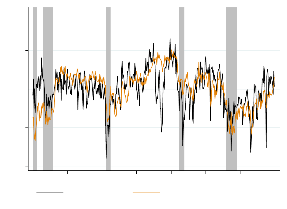
Figure 3: Sentiment Indexes Over Time

-4 -2 0 2 4

Standard Deviations

1980m1 1985m1 1990m1 1995m1 2000m1 2005m1 2010m1 2015m1

News Sentiment Consumer Sentiment (Michigan)

Notes: Shown are the point estimates of the time dummies (in months) for the news sentiment measure

(black line) and the University of Michigan Consumer Sentiment Index (orange line). Both measures are

normalized to have mean equal to zero and standard deviation equal to one.

Figure 4: Eﬀect of Cumulating Daily News Sentiment Since Prior Survey Release

.5 1 1.5 2 2.5 3

Coefficient

4 5 6 7 8

t-Statistic

0 5 10 15

Days since release of Prior Final Michigan Release

t-Statistic Coefficient

Michigan Consumer Sentiment

.5 1 1.5 2 2.5 3

Coefficient

4 5 6 7 8

t-Statistic

0 10 20 30

Days since release of Prior Consumer Confidence Release

t-Statistic Coefficient

Conference Board Consumer Confidence

Notes: Plotted are the coeﬃcients and t-statistics of β

from estimating equation (4), with γ

restricted to

one, for alternative values of d.

Figure 5: Impulse Response of a Positive News Sentiment Shock on Economic Activity

-.4 -.2 0 .2 .4

Percent

0 12

Horizon

Consumption

-1 -.5 0 .5 1

Percent

0 12

Horizon

Output

-.4 -.2 0 .2 .4

Percentage points

0 12

Horizon

Real rate

-.1 -.05 0 .05 .1

Percent

0 12

Horizon

Price level

Notes: Plotted are impulse responses from a news sentiment shock. The real rate is measured by the federal

funds rate, consumption is measured by real personal consumption expenditures (PCE) produced by the

Bureau of Economic Analysis (BEA), inﬂation is measured as the logarithm of the PCE price index (also

produced by the BEA), and output is measured by the industrial production (IP) index produced by the

Federal Reserve. The news sentiment shock is constructed as the component of the news sentiment series

that is orthogonal to current and 6 lags of economic activity as well as 6 lags of itself (in months). Plotted

are the point estimates, 68 (light grey), and 90 (dark grey) percent conﬁdence bands.

Appendix

A Details on Survey-Based Sentiment Indexes

A.0.1 Michigan Consumer Sentiment

The University of Michigan’s Consumer Sentiment Index (MCSI) dates back to the late

1940s.

It is based on a monthly telephone survey of at least 500 respondents across the

U.S. The index is constructed as a normalized sum of the relative scores (percent of responses

that are favorable minus percent of responses that are unfavorable) from the following ﬁve

questions:

(1) “We are interested in how people are getting along ﬁnancially these days. Would you

say that you (and your family living there) are better oﬀ or worse oﬀ ﬁnancially than you

were a year ago?”

(2) “Now looking ahead–do you think that a year from now you (and your family living

there) will be better oﬀ ﬁnancially, or worse oﬀ, or just about the same as now?”

(3) “Now turning to business conditions in the country as a whole–do you think that

during the next twelve months we’ll have good times ﬁnancially, or bad times, or what?”

(4) “Looking ahead, which would you say is more likely–that in the country as a whole

we’ll have continuous good times during the next ﬁve years or so, or that we will have periods

of widespread unemployment or depression, or what?”

(5) “About the big things people buy for their homes–such as furniture, a refrigerator,

stove, television, and things like that. Generally speaking, do you think now is a good or

bad time for people to buy major household items?”

A.0.2 Conference Board Consumer Conﬁdence

The Conference Board’s Consumer Conﬁdence index (CBCI) dates back to 1967 and is based

on their Consumer Conﬁdence Survey. Since 1977, this survey has been conducted monthly.

The Conference Board aims to get responses from roughly 3,000 households. Similar to

the Michigan index, the CBCI is based on the responses to ﬁve survey questions. The ﬁrst

Further details about the Michigan Consumer Sentiment index and the underlying survey can be found

at: https://data.sca.isr.umich.edu.

two questions relate to current business conditions and current employment conditions. The

other three questions relate to expectations of business conditions, employment conditions,

and family income six months ahead.

B Examples of Scored Newspaper Articles

B.1 Article 1: Positive Human Rating, Positive Model Score

“Stocks Surge to Records” (The Washington Post, July 10, 1999)

Stocks sailed to record highs today as continued optimism about corporate proﬁts and strong consumer

spending oﬀset the eﬀects of a rocky bond market.

The Dow Jones industrial average rose 66.81, to 11,193.70, topping its previous record close of 11,187.36,

set Wednesday. The Dow was up 54.46, or 0.49 percent, for the week.

The Standard & Poor’s 500-stock index and the Nasdaq composite index also set records. For the

Nasdaq, rich with technology stocks, today was the sixth record-setting day in seven sessions as it rose 21.21

to close at 2793.07. The S&P 500 rose 8.86, to 1403.28.

Stocks have been ﬂourishing as the ﬁrst few companies to report second-quarter earnings meet Wall

Street’s high expectations. With the robust economy continuing its expansion, analysts are predicting the

strongest proﬁt growth since the third quarter of 1997.

Dell Computer led technology issues, rising 2 7/8, to 42-13/16, after Goldman Sachs raised its rating on

the company. Analysts said the positive evaluation from Goldman sparked interest in the whole technology

sector, helping the Nasdaq extend its winning streak.

The Dow’s gain would have been much more modest without McDonald’s, which rose 3-15/16, to 44-

9/16. Wall Street investment ﬁrm Schroder & Co. upgraded the company’s stock, citing strong expectations

for the fast-food chain’s second-quarter sales.

DuPont rose 3-3/16, to 71-11/16, after the company unveiled some details of the spinoﬀ of its Conoco

unit.

Despite the solid gains, stocks were somewhat unsettled by continuing ﬂuctuations in the bond market.

Early in today’s session, stocks fell along with bond prices as the credit markets absorbed an $8.6 billion

oﬀering by Ford Motor and its Ford Motor Credit unit. The oﬀering is the largest corporate bond deal ever,

topping AT&T’s $8 billion sale earlier this year.

Prices evened out as the market digested the oﬀering. The yield on the Treasury’s 30-year bond, which

had risen as high as 6.03 percent at noon, edged back to 6 percent, which was up slightly from the 5.99

percent level it was at late Thursday. The long bond’s price fell $1.56 per each $1,000 invested.

Stocks recovered, although it was a quiet summer Friday with little news to stimulate trading. Advancing

issues outnumbered decliners by 18 to 11 on the New York Stock Exchange, where volume came to 701 million

shares, down from 830.6 million on Thursday.

The NYSE composite index rose 3.63, to 657.68; the American Stock Exchange composite index rose

4.04, to 812.73; and the Russell 2000 index of smaller companies rose 3.23, to 457.98.

Human Rating: 5 (Very Positive), GI: 0.02, HL: 0.03, LM: 0.01, Winning Model: 0.06

B.2 Article 2: Positive Human Rating, Negative Model Score

“Big Savings On Mortgages” (The San Francisco Chronicle, December 24, 1991)

The drop in mortgage rates is one of the most welcome changes resulting from the Federal Reserve

Bank’s cuts in the discount rate. Many families with a $150,000 mortgage can expect to save $100 a month

or more in house payments – far more than they could get from the tax programs presently being discussed

by Congress and the administration.

Such unencumbered savings should have far fewer negative side eﬀects than some of the current proposals

for tinkering with federal tax laws. Both parties agree that some revision of the nation’s tax code is advisable,

but it would be risky to increase the deﬁcit unnecessarily.

When homeowners’ disposable income rises, there is no such problem.

Frank Schultz, an executive vice president of Bank of America told Chronicle staﬀ writer Laura Evenson

that it is still too early for the savings consumers have realized from lower interest rates to be translated into

purchases. But the extra money will inevitably be available, both for increasing the sales of automobiles,

furniture, appliances and other major items and for reducing consumer debt.

In fact, consumer debt has already declined by 5.7 percent from last year’s ﬁgure of $388 billion.

What the change will mean for pension funds and other investors in the secondary mortgage market is

more diﬃcult to calculate. Their income will drop, but so will the cost of money they need to operate.

It is too early to tell when the recession will end. But getting mortgage rates under control is a sound

ﬁrst step.

Human Rating: 5 (Very Positive), GI: -0.03, HL: -0.01, LM: -0.02, Winning Model: -0.08

B.3 Article 3: Negative Human Rating, Negative Model Score

“U.S. Trade Gap Hits Record $19.4 Billion” (The Los Angeles Times, April 21, 1999)

Americans’ insatiable appetite for imported goods, along with weak overseas demand for U.S. products,

combined to produce a record $19.4-billion trade deﬁcit in February, the Commerce Department said Tuesday.

The deﬁcit has soared as the U.S. economy increasingly has become an island of prosperity amid a global

slowdown. Economic growth here has meant a strong domestic market for imports, while the slowdown

abroad has cut into oﬀshore sales of U.S. producers.

“It’s a simple story. You have the U.S. economic train going fast and no one can stop it. On the other

hand, economies in Latin America and Asia are slowing down or mired in recession,” said Fernando Losada,

senior economist at ING Barings in New York.

But the size of February’s deﬁcit, up from January’s revised deﬁcit of $16.8 billion, also a record, exceeded

expectations, mainly because the spending binge by U.S. consumers has exceeded anyone’s expectations.

Imports rose to $96 billion in February from $93.9 billion in January. Imported consumer goods, especially

autos, led the way.

Much of the added imports came from Japan, Mexico and Europe, causing U.S. deﬁcits with those

regions to widen further. But exports declined slightly to $76.6 billion from $77.1 billion in January, with

most of the slippage due to a decline in airplane shipments from Boeing Co. Aircraft shipments alone fell

by nearly $1 billion, adding to declines in food, automotive and industrial supplies.

“This is the ﬂip side of a domestic economy that’s ﬂying,” Salomon Smith Barney economist Brian Jones

said.

The U.S. economy seems to be defying gravity and the problems of its trading partners. Observers have

repeatedly had to upgrade their forecasts of U.S. economic activity.

Driving that growth is the estimated 6% surge in consumer spending so far this year, a reﬂection of high

consumer conﬁdence, low unemployment and $1 trillion in stock market proﬁts over the quarter, said Bruce

Steinberg, chief economist at Merrill Lynch in New York.

“As the U.S. economy continues to chug merrily along, others are hurting, so it shouldn’t come as a

surprise there is a trade deﬁcit,” said Brink Lindsey of the Cato Institute.

But there is a downside to continued deﬁcits if they persist, which is likely. Some economists warn that

the deﬁcit is impeding U.S. domestic economic growth by pushing sales and jobs oﬀshore.

“The trade sector is mitigating the strength of the U.S. economy,” Goldman Sachs economist John

Youngdahl said. Moreover, the growing imbalance has already rekindled protectionist sentiment in Congress.

The House earlier this year passed a measure to restrict foreign steel imports.

Federal Reserve Chairman Alan Greenspan this month warned that growing protectionism threatens the

country’s economic well-being.

But the near-record-low unemployment levels enjoyed by American workers has so far tended to defuse

the anti-import lobby.

And the widening trade deﬁcit has not yet weakened the U.S. dollar, which is a risk of widening trade

gaps, said William Stevenson, senior portfolio manager at Montgomery Asset Management in San Francisco.

The global economic malaise has only made U.S. dollars more desirable to hold, he said.

For now, most economists are resigned to the deﬁcit as an inevitable outgrowth of a global economy in

which the U.S. is clearly lapping its trade partners. What’s needed to rekindle demand for U.S. goods is a

global recovery.

The deﬁcit with Japan, the second-biggest U.S. commercial partner behind Canada, widened to $5.3

billion in February from $4.7 billion in January and $5.3 billion in February 1998.

The deﬁcit with Asia’s newly industrialized countries rose to $1.8 billion in February from $1.6 billion

in January and $885 million in February 1998.

A narrowing of the deﬁcit with China in February was good news for the Clinton administration’s eﬀorts

to strike a trade deal that would enable the Chinese to join the World Trade Organization.

But so far this year, the gap with China totals $9.5 billion, up sharply from $7.7 billion in the year-earlier

period. The deﬁcit with Canada decreased to $2.4 billion in February. The deﬁcit with Mexico widened to

a record $1.8 billion. The deﬁcit with Western Europe increased to $2.2 billion.

Human Rating: 1 (Very Negative), GI: -0.02, HL: -0.004, LM: -0.04, Winning Model: -0.10

B.4 Article 4: Negative Human Rating, Positive Model Score

“State is Losing Edge in Median Incomes” (Minneapolis Star Tribune, September 9, 2012)

Workers need more education to ﬁll high-wage jobs.

If you’ve lived in this state for more than a few years, the Minnesota you know is a place where educational

attainment and median household income are well above the national average. It’s a place where the quality

of life gets a boost from those higher incomes as they are donated and taxed in ways that keep schools good,

crime low, nature unspoiled, and arts and amenities ﬂourishing.

Evidence is mounting that in the wake of the Great Recession, Minnesota’s income advantage over the

rest of the nation is shrinking. The latest: A Star Tribune analysis of state labor data shows that the portion

of jobs paying $10 to $25 an hour has dropped sharply in the past decade, from nearly two-thirds of all job

postings in 2002 to 43 percent today. Meanwhile, more than a third of today’s openings are for jobs paying

less than $10 an hour.

That’s in keeping with the latest U.S. Census Bureau analyses putting Minnesota’s median household

income at $57.820 in 2011. While that’s still 15.5 percent above the national median, and represents a gain

from Minnesota’s 6.3 percent advantage in 2010, the state stood 29.2 percent above the national level on the

same measure in 2000.

Does that mean that Minnesota’s quality of life is at risk? Yes, said recently retired state demographer

Tom Gillaspy, if Minnesota doesn’t move aggressively to take advantage of the ﬂip side of the postrecession

employment trend. That side is also evident in the Star Tribune analysis: Jobs paying at least $25 an hour

have grown from 4 percent of Minnesota vacancies in 2002 to 19 percent in 2012. (These ﬁgures are adjusted

for inﬂation.)

The recession has accelerated a workforce trend that Gillaspy and his research partner, state economist

Tom Stinson, have long forecast. Generic, middle-income, middle-management jobs are disappearing as

enterprises learn to function with fewer of them. Low-skill, low-wage jobs are again in demand now, but

many remain in jeopardy of replacement by technology. If robots can do a job, they will, and soon.

But workers with specialized skills and the capacity to be both analytic and creative ”can name their

price” in many ﬁelds, Gillaspy said.

Securing more of those high-wage jobs and the beneﬁts their incomes provide means improving Min-

nesota’s educational attainment. Other states and nations are catching up to the educational advantage

Minnesota built for itself in the last half of the 20th century.

To stay above average in income and the rest, Minnesota needs another major leap forward in educational

attainment in the next decade. The 20th-century K-12 educational norm should give way to an expectation

that every youngster will experience formal learning from prekindergarten through ”grade 14” – that is, at

least two years of postsecondary study.

This state’s leading higher educators have been busy in the last year devising strategies for increasing

post-high-school educational attainment. But they can’t do the job alone. Enrolling more 4- and 5-year-olds

in quality preschools must also be part of a grand plan. So must a better, more individualized melding of

high school with college study and communitywide eﬀorts to keep youngsters in school.

All this eﬀort needs an orchestrator to coordinate and harmonize it – and there’s no one better positioned

for the task than Gov. Mark Dayton. Minnesota needs a new grand plan for success in the new economy.

As Dayton stumps the state for his party’s candidates this fall, we hope he is also gathering ideas and steam

for the strategic planning exercise that the 2013 legislative session should include.

Human Rating: 2 (Negative), GI: 0.04, HL: 0.02, LM: 0.02, Winning Model: 0.05

Figure A1: IRF with Michigan Consumer Sentiment Index Control

-.4 -.2 0 .2 .4

Percent

0 12

Horizon

Consumption

-1 -.5 0 .5 1

Percent

0 12

Horizon

Output

-.4 -.2 0 .2 .4

Percentage points

0 12

Horizon

Real rate

-.1 -.05 0 .05 .1

Percent

0 12

Horizon

Price level

Figure A2: IRF with Conference Board Consumer Conﬁdence Control

-.4 -.2 0 .2 .4

Percent

0 12

Horizon

Consumption

-1 -.5 0 .5 1

Percent

0 12

Horizon

Output

-.4 -.2 0 .2 .4

Percentage points

0 12

Horizon

Real rate

-.1 -.05 0 .05 .1

Percent

0 12

Horizon

Price level

Notes: Plotted are impulse responses from a news sentiment shock with additional controls. Panel A reports

the news sentiment shock constructed as the component of the news sentiment series that is orthogonal to 6

lags of itself, current and 6 lags of economic activity, current and 6 lags of the Michigan consumer sentiment

index. Panel B reports the news sentiment shock constructed as the component of the news sentiment

series that is orthogonal to 6 lags of itself, current and 6 lags of economic activity, current and 6 lags of

the Conference Board’s consumer conﬁdence index. Plotted are the point estimates, 68 (light grey), and 90

(dark grey) percent conﬁdence bands.

C Details of LASSO Estimation

We ﬁrst use a general LASSO model, which selects parameters without additional restric-

tions. The general LASSO is deﬁned as:

β = arg min

i=1

−

j=1

i,j

+ λ

j=1

| (7)

where y

represents the forecasted economic outcome of interest i, and x represents variables

of interest.

The optimal penalty parameter λ* for each y

is chosen based on a cross-validation

procedure. We choose λ* such that it yields the minimum out-of-sample RMSE across a

series of rolling 20-year-sample regressions. That is, we do a grid search over possible values

of λ, and for each possible λ we estimate the general LASSO model for each 240-month

sample (rolling from initial month of October 1986 to initial month of December 1996) and

collect the 12-month ahead forecast error. We then calculate, for each possible λ, the RMSE

across the 123 rolling samples. λ* is the λ yielding the minimum RMSE.

Last, we estimate the general LASSO model using the penalty parameter λ* and the full

sample to see which parameters are selected as useful predictors. If any of the parameters

(contemporaneous or lag) for each economic, survey, or news sentiment measure are chosen

as predictors in the general LASSO model, it is shown in Table 1.

We next use an adaptive LASSO model, which is a weighted variation of the general

LASSO model. The adaptive LASSO is deﬁned as:

β = arg min

i=1

−

j=1

i,j

+ λ

j=1

| (8)

where w

is a known weights vector such that ˆw = 1/|

β|. This variation of the general

LASSO model has oracle properties when λ is properly chosen.

Like in the general LASSO model, λ* is chosen such that it yields the minimum out-

of-sample RMSE across a series of rolling 20-year-sample regressions. For each 240-month

sample we calculate a separate weights vector, which requires a second cross-validation pro-

cedure. On each 240-month sample we estimate a series of rolling 8-year-sample regressions

for

λ corresponding to the 240-month sample and collect the 12-month ahead forecast error.

We then calculate for each possible

λ the RMSE across the 133 rolling samples.

λ* is the

λ yielding the RMSE. The coeﬃcients corresponding to

λ are

β and are used to calculate

ˆw. We re-scale each 240-month sample and for each possible λ estimate the general LASSO

model on each sample (rolling from initial month of October 1986 to initial month of Decem-

ber 1996) and collect the 12-month ahead forecast error. We then calculate, for each possible

λ, the RMSE across the 123 rolling samples. λ* is the λ yielding the minimum RMSE.

With λ*, we estimate the general LASSO model on the full sample to see which pa-

rameters are useful predictors. If any of the parameters (contemporaneous or lag) for each

economic, survey, or news sentiment measure are chosen as predictors in the general LASSO

model, it is shown in Table 1.

For the last exercise, we estimate the group LASSO model which forces groups of param-

eters to zero simultaneously. The group LASSO is deﬁned as:

j,λ

= arg min(||Y

− X

+ λ

g=1

||β

) (9)

where Y

represents the forecasted economic outcome of interest j. X is the design matrix

and I

is the index for the gth group of variables. We consider a “group” to be a the block

of the contemporaneous value and 12 lags of each variable.

The optimal penalty parameter λ* is chosen, separately for each forecasted outcome (Y

based on a cross-validation procedure. We choose λ* such that it yields the minimum out-

of-sample RMSE across a series of rolling 20-year-sample regressions. That is, we do a grid

search over possible values of λ, whereby for each possible λ we estimate the group LASSO

model for each 240-month sample (rolling from initial month October 1986 to initial month

December 1996) and collect the 12-month ahead forecast error. We then calculate, for each

possible λ, the RMSE across the 123 rolling samples. λ* is the λ yielding the minimum

RMSE.

Lastly, we estimate the group LASSO model using the penalty parameter λ* and using the

full sample to see which ”groups” (economic outcome, survey, and news sentiment measures)

are selected as being useful predictors. The groups chosen as predictors in the group LASSO

model are shown in Table 1.