
1
How Essential Is Essential Air Service?
The Value of Airport Access for Remote Communities
Austin J. Drukker
University of Arizona
May 2023
Essential Air Service is a federal government program that provides subsidies to airlines that
provide commercial service between certain remote communities and larger hubs, which
proponents argue are justified because driving to larger airports would be prohibitively
expensive for residents of these communities. I estimate the value of Essential Air Service to
local communities using a revealed-preferences approach by formulating and estimating a
discrete-choice model of domestic air travel purchases that incorporates passengers’
geographical proximity to alternative airports. I estimate the model using proprietary data
containing millions of domestic airline passengers’ residential ZIP codes coupled with their
choice of airline product. Simple data tabulations reveal that most travelers living in regions
receiving subsidized service have several alternative airports to choose from and generally
prefer to drive to larger airports. A counterfactual policy simulation using the estimated model
finds that, in aggregate, community members value subsidized commercial air service from
their local airport at $16 million per year, compared to an annual cost of over $290 million.
Keywords: airport, airline, subsidy, public finance, substitution, discrete choice
JEL Codes: H54, L93, R53
I. INTRODUCTION
For the last half century, the US domestic aviation industry has operated in a largely unregulated market
environment. The Airline Deregulation Act of 1978 removed federal government control over fares, routes,
flight frequency, and the entry of new airlines, leading to improvements in service, decreases in fares, and
increases in the number of flights, passengers, and miles flown. Today, passenger aviation is a major
component of the modern global economy, contributing about 5 percent to US gross domestic product
annually (IATA, 2019; FAA, 2020). According to the International Civil Aviation Organization, 4.5 billion
passengers globally flew on scheduled air service in 2019, and the Federal Aviation Administration (FAA)
provides air traffic control services for more than 2.9 million airline passengers per day (FAA, 2022).
According to the Consumer Expenditure Survey, about 13 percent of US households purchased at least one
airline ticket in 2019 and spent an average of $3,873 on airfare.
Although the Airline Deregulation Act was largely viewed as a success, there was fear among some at
the time of its passage that small communities would be left behind in its wake as airlines shifted their
operations to serve large, profitable markets. To assuage this fear, Congress established Essential Air
Service (EAS) in 1978, which required carriers to continue providing scheduled air service at pre-

2
deregulation levels—typically two round trips per day—to eligible communities using subsidies if
necessary. Although EAS was originally set to expire after 10 years, under the assumption that air traffic
would eventually become self-sustaining, Congress reauthorized EAS for another 10 years in 1988 and
made it permanent in 1996. As of June 2022, costs for the program have ballooned to over $340 million
per year despite fewer communities being eligible today compared to in 1978. Given that EAS still exists
nearly a half century after Congress originally intending it to expire, it is reasonable to ask whether EAS
still achieves its stated purpose of efficiently and effectively connecting remote communities to commercial
air travel opportunities.
1
Understanding the value of EAS to the communities it serves requires understanding the trade-offs
faced by travelers. A key trade-off that community members face is whether to fly from their local airport,
which may be more convenient but offer fewer choices, or to drive to a larger airport, which may be far
away but offer more choices. To study this trade-off, I analyze proprietary choice data derived from credit
card transactions that link travelers’ airline product choices with their home ZIP code. The data, which have
not been used in any previous economic studies, allow me to easily compute travelers’ driving time to
alternative airports.
2
Hence, driving time is an observable product characteristic whose marginal value to
consumers can be estimated using standard econometric techniques.
The proprietary choice data reveal several important insights about airline markets previously not
known to researchers and policymakers. First, since I am able to directly observe which airports are chosen
by residents of a particular geographical area, it is relatively straightforward to determine which airports
effectively serve the same region.
3
While the presence of multiple airports in a region does not in itself
imply that the airports provide substitutable services, the growth of air travel demand since the early 1990s
has attracted entry by airlines at different airports within the same region, suggesting a potentially important
role for spatial interactions in the airline industry that have been largely overlooked by previous research.
4
1
The Airline Deregulation Act (92 Stat. 1733) requires the Department of Transportation to “consider the desirability
of developing an integrated linear system of air transportation whenever such a system most adequately meets the air
transportation needs of the communities involved.”
2
To my knowledge, only two academic papers (Yirgu and Kim, 2021; Yirgu, Kim, and Ryerson, 2021) have used
these data, and both papers use only a small geographical subset, in contrast to my data sample which covers the entire
United States from 2013 to 2019.
3
See Fournier, Hartmann, and Zuehlke (2007). Studies that have considered regions with multiple airports vary widely
in which airports to include. Berry and Jia (2010, p. 11) consider six regions to have airports that are “geographically
close.” de Neufville (1995) lists nine regions served by more than one airport. Brueckner, Lee, and Singer (2014)
attempt to empirically estimate which airports serve the same metropolitan region based on competition spillovers and
specify 13 regions as having multiple competing airports. Drukker and Winston (forthcoming) consider 22 regions to
have multiple competing airports.
4
Studies that consider aspects of spatial competition in non-airline markets include Manuszak and Moul (2009) and
Dorsey, Langer, and McRae (2022) (gasoline); Smith (2004) and Katz (2007) (supermarkets); Davis (2006) (movie
theaters); Ho and Ishii (2011) and Hatfield and Wallen (2022) (banking); and Murry (2017) and Murry and Zhou
(2020) (car dealerships). Studies that consider aspects of spatial competition in airline markets include Fournier,

3
Relatedly, since I am able to observe the home ZIP code of an airport’s users, it is relatively
straightforward to determine the geographical boundary of an airport’s catchment area (the area from which
an airport draws its customers). Administrative and survey data from a variety of sources suggest that most
airports draw customers from a large geographical area, but most previous studies of the airline industry
have assumed airports have relatively small catchment areas, typically the geographical boundaries of a
city.
5
Proper market definition is of first-order concern for almost any industry analysis because it directly
influences the scope of available substitutes for consumers and the degree of competition faced by suppliers.
Excluding certain viable airports from travelers’ choice sets may rule out important substitution patterns,
and estimates derived from narrowly defined choice sets will tend to overstate airlines’ market power by
understating travelers’ ability to substitute to alternative products, which in turn could have significant
implications for merger evaluations and antitrust enforcement.
6
The ability to view travelers’ choice sets is particularly useful for evaluating the costs and benefits of
EAS, since implicit in much of the debate surrounding the program is the assumption that members of
communities receiving EAS-subsidized service would have no other viable alternatives for accessing
commercial air travel apart from subsidized service from their local airport. My choice data allow me to
see which airports residents of an arbitrary geographical area actually use, allowing me to directly check
this assumption.
7
Simple tabulations of the proprietary choice data reveal a key insight about the nature of
EAS community members’ choice sets, namely, that despite their ostensible isolation from the rest of the
national air transportation system, members of most EAS communities rarely choose to fly on EAS-
subsidized flights from their local airport and instead generally prefer to drive to airports of various sizes
offering more products with better characteristics. From an econometric perspective, failing to consider
these viable alternatives in travelers’ choices sets will make EAS appear more valuable than it actually is
because travelers will appear less price sensitive due to having fewer substitutes. From a policy perspective,
Hartmann, and Zuehlke (2007), Hess and Polak (2005, 2006), Ishii, Jun, and Van Dender (2007, 2009), Mahoney and
Wilson (2014), Brueckner, Lee, and Singer (2014), McWeeny (2019), and Drukker and Winston (forthcoming).
5
Airlines For America’s 2019 annual survey found that 37 percent of passengers reported flying from an airport that
was not the closest to their home or office at some point in the previous year. McWeeny (2019) found that a significant
share of travelers surveyed at San Francisco International Airport drove from as far away as Sacramento (a 2-hour
drive) and that 57 percent of passengers surveyed at San Francisco International Airport bypassed an airport that was
closer to their home. Ishii, Jun, and Van Dender (2007) found that travelers located closest to San Francisco
International Airport most often departed from there, but passengers closest to San Jose International Airport or
Oakland International Airport often chose to fly from a different airport. Yirgu, Kim, and Ryerson (2021) report
significant airport leakage for small and medium-sized airports in the Midwest United States.
6
The US Department of Justice uses a narrow city-pair market definition in cases involving airline mergers. See, for
example, their complaint against the proposed merger between American Airlines and US Airways (78 Fed. Reg.
71377) and their complaint against the Northeast Agreement between American Airlines and JetBlue Airways
(https://fingfx.thomsonreuters.com/gfx/legaldocs/zjpqkrdlmpx/plaintiffs-brief-american-airlines-2022.pdf).
7
Bao, Wood, and Mundy (2015) and Lowell et al. (2011) compute the cost of subsidizing flights to the cost of
subsidizing bus service to the same location. They do not consider the costs of subsidizing bus service to alternative
airports.

4
the revelation that EAS community members frequently choose to drive to alternative airports undermines
EAS’s raison d’être to provide an essential service to communities that would otherwise have no other
options to connect to the national air transportation system.
8
An added benefit of the proprietary choice data is that I can see the home location of any airport’s users,
which allows me to determine the extent to which an EAS-subsidized airport serves residents of the
community. Knowledge of the home location of EAS-subsidized airport users is policy relevant because
the purpose of EAS is to connect residents of the community to commercial air travel. Without the ability
to link purchases to the home location of purchasers, it would not be possible to determine who are the
primary users of EAS-subsidized service. Tabulations of the data reveal that the majority of EAS-subsidized
airport users are not residents of the communities in which the airport is located. This finding has important
fiscal policy implications because all users of EAS airports benefit from subsidized ticket prices, regardless
of residency status, implying a majority of EAS funds go toward subsidizing nonresidents of EAS
communities. The problem is further compounded by the fact that nonresidents who use EAS-subsidized
airports tend to have higher incomes than residents, which raises serious distributional concerns about the
program.
To formally estimate the value that EAS community members derive from the program, I formulate
and estimate a discrete-choice model of air travel demand. I formulate my demand model using a nested
logit utility specification that closely resembles the canonical models of Berry, Carnall, and Spiller (1996,
2006) and Berry and Jia (2010). A key component of my model is the inclusion of driving time as a product
characteristic, which allows me to directly estimate the implicit monetary costs of driving to alternative
airports. I estimate my model using the generalized method of moments with a combination of macro and
micro data, as described by Berry, Levinsohn, and Pakes (2004) and Petrin (2002). Macro moments are
constructed using aggregate data containing information about airline products, their characteristics, and
the number of travelers who choose each product, and micro moments are constructed using the proprietary
choice data. Intuitively, the micro moments capture spatial variation between driving time and travelers’
choices (and non-choices), which is used to identify travelers’ preferences for driving.
9
A useful feature of the discrete-choice modeling framework is that it allows me to analyze
counterfactual policy experiments by estimating consumer surplus under two alternative scenarios. In
particular, I consider a counterfactual policy experiment in which all EAS subsidies are eliminated, which
8
Grubesic and Matisziw (2011) thoroughly studied EAS community members’ access to a variety of alternative
airports, but their data do not allow them to study the extent of their use.
9
McWeeny (2019) uses a similar revealed-preferences approach, which, unlike the stated-preferences approach used
by Landau et al. (2016), Daly, Tsang, and Rohr (2014), Adler, Falzarano, and Spitz (2005), Hess and Polak (2006),
Merkert and Beck (2017), and Hess, Adler, and Polak (2007), does not rely on self-reported or speculative valuations
of trip components.

5
would cause commercial service to cease at most airports currently served by EAS-subsidized airlines. The
difference between consumer surplus computed before and after the elimination of commercial service at
EAS airports reveals community members’ implicit value of the EAS program, and a simple comparison
between the costs and benefits of the program can be used to determine whether EAS subsidies are justified.
I conduct my counterfactual policy experiment using data from 2019 for 107 EAS communities in the
continental United States. The analysis reveals that the members of these 107 communities collectively
value subsidized service from their local airport at $16 million annually, a paltry amount compared to EAS’s
cost in 2019 of over $290 million. Furthermore, this estimate likely overstates the effects of eliminating
EAS subsidies, since commercial service might not cease at all formerly eligible communities.
Disaggregating the results by airport reveals that desirable routes tend to be flown by legacy airlines
operating in a seemingly competitive environment, which is suggestive of rent-seeking behavior to the
extent EAS subsidies act as entry barriers for competitors.
The remainder of this paper is organized as follows. In Section II, I provide a brief history and overview
of Essential Air Service. In Section III, I describe my data and present several novel insights based on
descriptive statistics. In Section IV, I formulate an empirical model of demand, and in Section V, I describe
the estimation strategy and sources of identification. In Section VI, I present the estimation results and
perform post-estimation checks. In Section VII, I present the results of my counterfactual policy analysis
to compute the consumer surplus that communities derive from EAS and consider distributional
implications. Section VIII concludes with a summary of the findings, policy recommendations, and
suggestions for future research.
II. ESSENTIAL AIR SERVICE
The EAS program provides subsidies to airlines to provide regular service to eligible communities.
10
,
11
To be eligible for EAS, a community must be located more than 70 miles from the nearest medium or large
hub airport, require a per-passenger subsidy rate of $200 or less ($1,000 or less if the community is farther
than 210 miles from a hub), and have 10 or more enplanements per day.
12
EAS typically subsidizes one
airline to provide two to four round trips per day, six days per week, from an EAS community to a larger
hub. Although EAS eligibility is based on a community’s distance to the nearest medium or large hub,
10
A handful of communities participate in the Alternate EAS program, which allows communities to forgo traditional
EAS for a prescribed amount of time in exchange for a flexible grant. In 2019, all communities participating in the
Alternate EAS used their funds to subsidize charter air service.
11
EAS contracts do not give an airline the exclusive right to serve a community, and airlines may decide to serve a
community under an EAS contract without the use of subsidies.
12
See Appendix C for a summary of the legal statutes and DOT practice regarding eligibility determination. Tang
(2018) provides an excellent primer on EAS, its history, and eligibility requirements.

6
airlines that receive EAS contracts are not required to fly passengers to the nearest hub nor to a medium or
large hub.
13
Airlines compete for EAS contracts through a bidding process, and the DOT typically receives 1–3
proposals per airport every 1–3 years, when EAS contracts typically expire. By law, the DOT must take
into account the views of the community when deciding which proposal to accept, as well as the carrier’s
service reliability and any arrangements it has with larger carriers at the hub. Notably, subsidy cost is not
among the factors the DOT is required by law to consider when evaluating bids, and if more than one carrier
proposes to offer service then local officials are under no obligation to favor the proposal that entails the
lowest cost to the federal government.
EAS has long been a target of critics who have derided the program as wasteful spending and an
inefficient means of connecting rural communities to commercial air travel, arguing that the statutes
governing EAS do not encourage cost efficiency and that the market, not government subsidies, should
decide which airports survive. But community stakeholders argue that EAS provides an essential service to
communities that would otherwise lose access to commercial air travel, arguing that EAS community
members value their local airport and without government subsidies the airport would cease to be
commercially viable. Several papers have argued that ending EAS subsidies would not necessarily reduce
service at eligible communities.
14
But the question of whether and the extent to which EAS community
members value their local airport has not been studied and is one that I take up in the present paper.
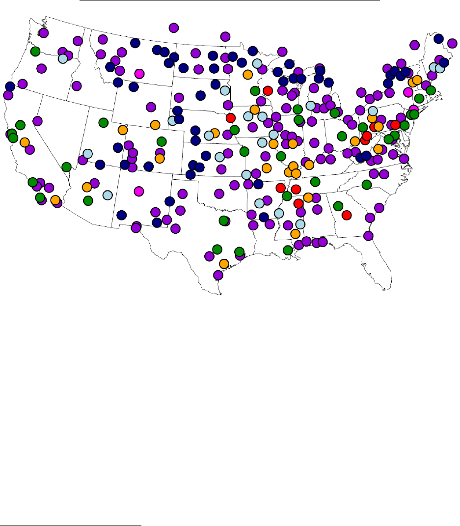
Figure 1 shows the locations of 107 airports receiving EAS-subsidized service as of September 2021.
15
Following the Eno Center for Transportation’s (2018) convention, red dots represent communities that are
between 70 and 100 miles from a medium or large hub, orange dots represent communities that are between
100 and 150 miles from a medium or large hub, light blue dots represent communities that are between 150
and 210 miles from a medium or large hub, and dark blue dots represent communities that are more than
210 miles from a medium or large hub (DOT, 2021c). The green dots correspond to medium or large hubs
that are nearest to EAS communities or which are used by airlines serving EAS communities even if not
geographically closest (DOT, 2019a, 2022b).
13
For example, Cape Air currently serves several EAS communities in Montana through their small hub at Billings
Logan International Airport. See Appendix C for the FAA’s definition of hub size.
14
Cunningham and Eckard (1987) suggest that EAS subsidies may have actually reduced flight frequency because
EAS contracts serve as entry barriers that discourage competition. Morrison and Winston (1986) note that service to
small communities actually increased following deregulation—suggesting EAS subsidies mask profit opportunities.
Bao, Wood, and Mundy (2015) note 10 of the 34 EAS communities that have had their EAS subsidies terminated
since 1993 have experienced a substantial increase in their outbound passenger levels. Furthermore, subsidized airlines
currently provide commercial service alongside unsubsidized airlines at several EAS airports, most notably Allegiant
Air, which serves five currently eligible communities and one formerly eligible community.
15
Appendix Table H3 lists the status of the 51 communities that have lost their EAS eligibility since 1989.

7
Figure 1. The Locations of EAS Airports and Their Nearest Hubs
Source: Federal Aviation Administration.
Notes: Green dots are medium or large hubs that are geographically closest to EAS communities or are
used by EAS-subsidized carriers. Red, orange, light blue, and dark blue dots are EAS airports located less
than 70 miles, 70–100 miles, 100–210 miles, and more than 210 miles, respectively, from the nearest
medium or large hub.
Although it would appear from Figure 1 that many EAS communities face considerable barriers to
access commercial air travel without the assistance of EAS, the color-coding belies the full picture by
restricting the notion of viability to medium hubs or larger. Figure 2 presents a fuller picture, augmenting
Figure 1 by including a host of viable airports that are classified as smaller than medium hubs. For example,
Figure 1 suggests Butte in southwest Montana is relatively isolated, located 6 hours to Salt Lake City to the
south and 10 hours to Portland or 9 hours to Seattle to the west. But Figure 2 reveals that there are four
additional airports within a 3-hour drive from Butte: Great Falls International Airport, Missoula Montana
Airport, Helena Regional Airport, and Bozeman Yellowstone International Airport, a small hub served by
8 major airlines flying to more than 20 destinations. The pink dots correspond to small hubs that are or have
8
been used by airlines to serve certain EAS communities, but which are too small to factor into the distance
calculation for maximum allowable per-passenger subsidies.
16
Figure 2. The Locations of EAS Airports and Viable Nearby Airports
Sources: Federal Aviation Administration; Airlines Reporting Corporation.
Notes: See the notes to Figure 1. Pink dots are small hubs that are or have been used by EAS-subsidized
carriers. Purple dots are airports used by a nontrivial share of EAS community members.
16
For example, Yellowstone Regional Airport in Cody, Wyoming, is only about 100 miles from Billings Logan
International Airport, but since Billings is considered a small hub it does not factor into the distance calculation; Salt
Lake City International Airport is the nearest large hub (about 450 miles away), so a carrier serving Yellowstone
Regional Airport would be exempt from the $200 per-passenger subsidy limit (DOT, 2019a).

9
III. DATA AND DESCRIPTIVE STATISTICS
Before describing the model and estimation strategy, I describe the data used to estimate the model and
present several figures showing the key features of the data. The data come from six primary sources. Table
1 (presented at the end of this section) provides summary statistics for several key variables.
A. Market Locator
The primary data set used for the analysis comes from the Airlines Reporting Corporation’s (ARC’s)
Market Locator tool. Owned by the airline industry, ARC acts as a clearing system for all travel agencies,
including online travel agencies such as Booking Holdings, Expedia Group, and their subsidiaries, which
process about 35 percent of all domestic tickets sold in the United States. According to ARC, the clientele
is representative of the universe of domestic leisure and unmanaged business travelers.
17
About 20 percent
of all tickets that come through the ARC clearing system are sent to a credit card processing company that
matches customers’ chosen product to their credit card billing ZIP code.
18
The data are associated with the
point of sale of the airline ticket purchaser, which is likely to be the passenger in most cases.
19
Thus, the
data are a roughly 7 percent representative sample of US domestic leisure passengers.
The Market Locator data contain monthly passenger counts by ZIP code for 2013–19. Tabulations of
the Market Locator data reveal which airports travelers drive to without a priori selecting which airports to
include in a traveler’s choice set. For example, Figure 3 shows the 8 airports most commonly chosen by
residents of Decatur, Illinois and their respective market shares. In 2019, Cape Air received $3.065 million
to offer 24 nonstop round trips per week to O’Hare International Airport (ORD) and 12 nonstop round trips
per week to St. Louis Lambert International Airport (STL) from Decatur Airport (DEC), with fares to
Chicago starting at $59 one way and fares to St. Louis starting at $29 one way (DOT, 2017, 2019a; Cape
Air, 2018). According to the DOT (2019a), Decatur Airport had 17,066 passengers (both directions) in
2019, corresponding to a $180 per-passenger subsidy. Despite Cape Air offering unusually low prices,
tabulations of the Market Locator data reveal that only 7 percent of travelers flew from Decatur to either
Chicago or St. Louis, while 21 percent of travelers drove 2 hours and 15 minutes to St. Louis, 27 percent
of travelers drove 3 hours to Chicago, and 27 percent of travelers drove 1 hour to Central Illinois Regional
17
As noted by Yirgu, Kim, and Ryerson (2021), business travelers are more inclined to purchase tickets directly from
airlines rather than through third-party agents, meaning they are less likely to show up in the Market Locator data.
18
The ability to link tickets with billing ZIP codes is only limited by the credit card processing company used for the
transaction; otherwise, there are no selection criteria for determining which tickets can be linked with billing ZIP
codes. The credit card processing companies generally do not process American Express cards, so there is a slight bias
against business travelers to the extent business travelers are more likely to pay with American Express cards.
19
Although the traveler’s point of origin is typically within proximity to the purchaser’s point of sale, this would not
be the case if, for example, the purchaser and passenger were in different locations or, more frequently, if the traveler
purchased one-way tickets individually.

10
Airport (BMI), a non-hub primary commercial service airport served by four major airlines. The remaining
travelers drove to Springfield’s Abraham Lincoln Capital Airport (SPI), Urbana–Champaign’s Willard
Airport (CMI), Indianapolis International Airport (IND), or Peoria International Airport (PIA).
Figure 3. Market Shares for Airports Chosen by Residents of Decatur
Source: Airlines Reporting Corporation.
Notes: See the notes to Figure 2. DEC is an EAS-subsidized airport in Decatur, Illinois. Market shares
conditional on flying are shown as percentages after the airport codes. The dotted lines indicate travelers
drove from Decatur to the indicated airport to take a departing flight. The dashed line indicates travelers
flew from DEC to the indicated airport en route to a final destination.
The Market Locator data are also useful for determining who the primary users of an EAS-subsidized
airport are, namely, residents of the community or nonresident visitors. Knowing the home location of an
EAS airport’s users is policy relevant because the purpose of EAS is to connect EAS community members
to commercial air travel. To determine the residency status of EAS airport users, I draw geographical
boundaries around the communities as shown in Appendix B—typically the Metropolitan or Micropolitan
Statistical Area(s) encompassing the airport. Residents are then defined as passengers whose ZIP code is
within the geographical region, and nonresidents are those whose ZIP code is outside the region. Overall, I
find that nonresidents make up 57 percent of customers on EAS-subsidized flights. As shown in Appendix

11
Figure H1 and Appendix Table H2, several EAS communities are located very close to national parks, and
airports in these communities likely serve as entry points for visitors; since all customers on EAS-
subsidized flights, regardless of where they live, benefit from lower ticket prices, it is plausible that EAS
serves to subsidizes tourism for these areas, which is not its statutory purpose. Yellowstone Airport, for
example, is used almost exclusively by tourists likely visiting Yellowstone National Park, while residents
of West Yellowstone overwhelmingly prefer to drive 1 hour and 30 minutes north to Bozeman Yellowstone
International Airport.
20
As will be explained in Section V.A, I use the Market Locator data to construct micromoments to be
used for generalized method of moments estimation of the parameters of interest. I thus restrict the sample
of Market Locator data in several ways. First, since several low-cost and ultra-low-cost carriers (including
Southwest Airlines and Allegiant Air) generally do not have contracts with travel agencies or are not
members of ARC, I do not observe travelers choosing products from these airlines.
21
I therefore restrict the
set of airlines to the four legacy carriers: American Airlines, Delta Air Lines, United Air Lines, and US
Airways.
Second, in order to identify substitution between airports, travelers living in an origin region must face
a choice set containing at least two airports. I therefore restrict the origin regions under consideration to
those among the top 40 busiest that contain at least two airports both served by a legacy carrier (see
Appendix Table H1). These include Boston, Chicago, Cincinnati, Cleveland, Dallas, Detroit, Houston, Los
Angeles, Miami, New York, Orlando, San Francisco, Tampa, and Washington, from which I drop Orlando
Sanford International Airport (SFB), Chicago Rockford International Airport (RFD), and St. Pete–
Clearwater International Airport (PIE) because these airports are not served by a legacy carrier.
22
Lastly, I must specify each airport’s catchment area in order to calculate market shares. Market shares
are defined as a given product’s share of the total potential trips from an origin area to a destination city.
Appendix A shows airport locations and the constructed catchment areas for the 40 busiest origin regions,
with darker shading corresponding to areas with higher population density. Appendix Table H1 shows the
land area of each catchment area and the passenger-weighted average drive time to passengers’ chosen
20
As noted by Grubesic and Wei (2013), Yellowstone Airport has the lowest subsidy rate among all EAS airports and
a sparse local population base but has a much higher load factor than the national average, likely due to tourism.
According to the National Park Service, approximately 1.73 million people used the west entrance to Yellowstone
National Park in 2019.
21
Southwest Airlines joined ARC in July 2019 and only shares data for corporate bookings made through its corporate-
client wing SWABIZ.
22
Although Southwest Airlines has nearly 100 percent market share at Chicago Midway International Airport (MDW),
Dallas Love Field (DAL), and Hobby Airport (HOU), the fact that legacy carriers have some market share at these
airports implies the micromoments can still identify the parameters under the generalized method of moments
estimation framework.

12
airport. The market size is assumed to be the total population of the catchment area, or the number of
potential passengers who consider air travel from an origin region to a destination city.
23
B. OpenStreetMap
Driving times between ZIP code centroids were extracted from OpenStreetMap using the Open Source
Routing Machine, a high-performance routing engine for shortest paths in road networks. The
OpenStreetMap data have an advantage over geodesic distance data (as the crow flies), such as the National
Bureau of Economic Research’s ZIP Code Distance Database, because they properly account for vehicle
mode, speed limits, and the nonlinear nature of road networks, although they do not account for delays
caused by traffic. Travel time is based on speed limits for different road types.
C. Airline Origin and Destination Survey
Product characteristics and market shares were constructed using the DOT’s Airline Origin and
Destination Survey (DB1B), a 10 percent quarterly sample of airline tickets from US carriers that contains
detailed itinerary information such as fares, layovers, and carrier identity. As noted in Section V.A, the
DB1B data is used to construct macromoments to be used for generalized method of moments estimation
of the parameters of interest. I consider flights departing from the 40 busiest origin regions and arriving at
the 100 busiest destinations for every quarter from 2013 to 2019, excluding origins in Hawaii, Alaska, and
Puerto Rico. Appendix Table H1 lists the 40 origin regions under consideration and the 76 airports
contained within them, as well as populations of the constructed catchment areas (see Appendix A). I
determine which airports belong in which regions largely based on the recommendations of Brueckner,
Lee, and Singer (2014).
I clean the DB1B sample following standard sample cleaning procedures from the literature:
24
I drop
all itineraries with more than one connection and collapse all coupons with a layover into a single
observation, regardless of the layover airport; the prices for such products (indirect flights) are computed
as the passenger-weighted average price. I drop all itineraries that start and end at different airports (i.e.,
are not round trips), are not economy class for all coupons, and are not flown on the same airline for all
coupons. I drop all itineraries with a fare of less than $11.20 (the September 11 Security Fee for a round-
23
Roughly speaking, market size is “some number of potential passengers who consider air travel” (Berry, Carnall,
and Spiller, 2006, p. 189). Although somewhat arbitrary, Berry, Carnall, and Spiller (2006, p. 189) note that the use
of the geometric mean of the origin and destination city populations as a measure of market size has “both empirical
and (weak) theoretical precedent in the literature on travel demand.” Population of the origin region is a reasonable
measure of market size in my context because my sample of aggregate data is constructed using round-trip tickets,
and passengers who desire to fly from an origin to a destination and back are much more likely to be residents of the
origin region as opposed to residents of the destination city.
24
My sample cleaning procedure closely follows the cleaning procedure described by Severin Borenstein
(http://faculty.haas.berkeley.edu/borenste/airdata.html).

13
trip ticket), such as those booked entirely with airline loyalty points, or greater than $2,500. In addition, I
only consider flights whose ticketing carrier is a reporting carrier, defined as a carrier with more than 0.5
percent of total domestic scheduled service passenger revenues; these include American Airlines, Delta Air
Lines, United Air Lines, US Airways, Southwest Airlines, JetBlue Airways, Alaska Airlines, AirTran
Airways, Virgin America, Allegiant Air, Frontier Airlines, Spirit Airlines, and Sun Country Airlines.
25
D. Airline On-Time Performance
Additional product characteristics such as flight frequency, extra flight time, and layover times were
constructed using the DOT’s Airline On-Time Performance data. Layover times are computed by assuming
passengers choose the itinerary with the shortest possible layover longer than a minimum connection time
of 30 minutes, which is the industry standard for US domestic flights.
E. Zip-Codes.com
Detailed ZIP code demographics were obtained from zip-codes.com’s ZIP Code Database (Business
edition). Several useful demographics included in the database are population (used to construct market
size), racial and gender composition, average home value, median household income, median age, and
congressional district. The data are compiled by zip-codes.com using data from the US Postal Service, US
Census Bureau, Office of Management and Budget, and various private sources.
Figure 4 shows the distribution of median household income for EAS communities alongside the
distribution of median household income for all Core-Based Statistical Areas (CBSAs), where a region’s
median household income is computed as the weighted average of median household incomes across ZIP
codes contained in the region. The median of the distribution for EAS communities is $52,500 compared
to $64,250 for all CBSAs, implying EAS communities generally have lower incomes compared to the
nation as a whole. Combining the demographic data with Market Locator data, Figure 5 shows the
distribution of median household income for users of EAS airports broken down by EAS community
residency status. Residents flying out of an EAS airport tend to have lower incomes than nonresidents flying
into an EAS airport—medians of the distributions $53,400 and $62,800, respectively. Thus, not only do the
majority of EAS funds go toward subsidizing nonresidents of the EAS community, but these nonresidents
also tend to have higher incomes than residents.
25
I exclude Hawaiian Airlines because it primarily serves Hawaii, which I exclude from my set of origin regions.
AirTran Airways merged with Southwest Airlines in May 2011 but was coded separately until January 2015. US
Airways merged with American Airlines in December 2013 but was coded separately until October 2015. Virgin
America merged with Alaska Airlines in April 2016 but was coded separately until April 2018. I classify large regional
carriers under their corresponding marketing carrier.

14
Figure 4. Distributions of Income for EAS Communities and All CBSAs
Source: zip-codes.com.
Note: The densities are constructed using an Epanechnikov kernel with a bandwidth of $5,000.
Figure 5. Distributions of Income for Resident and Nonresident EAS Airport Users
Sources: Airlines Reporting Corporation; zip-codes.com.
Notes: Median household income is based on the ZIP codes of passengers from Market Locator for 2013–
19. The densities are constructed using an Epanechnikov kernel with a bandwidth of $5,000.

15
F. American Community Survey
The American Community Survey (ACS) was used to construct income distributions at the ZIP code
level, as explained in Appendix E. The ACS contains information about the number of households living
in each Census block group with income in each of 16 income buckets ranging from $0 to $200,000 and
above. These data were used to construct income distributions at the ZIP code level using a block group to
ZIP code crosswalk obtained from the Missouri Census Data Center. The crosswalk, which provides the
share of the population of each block group that lives in each ZIP code, was used to allocate the number of
households in each block group into each ZIP code. Once block group populations were allocated to ZIP
codes, the total number of households in each ZIP code and income bucket was computed. Finally, the
number of households in each ZIP code and income bucket were converted to population shares by dividing
by the total population of the origin region.
Table 1. Summary Statistics for the Estimation Samples
Variable
Mean
Standard
deviation
Source
Fare (dollars)
186.69
66.87
DB1B
Direct
184.23
66.22
DB1B
Indirect
228.60
63.91
DB1B
Drive time (minutes)
38.4
21.1
Market Locator
Multi-airport region
38.3
21.6
Market Locator
Single-airport region
38.6
20.2
Market Locator
Extra time (minutes)
148
40
DB1B, On-Time
Layover time
83
32
DB1B, On-Time
Flight time
65
25
DB1B, On-Time
Number of daily flights
5.5
3.8
DB1B, On-Time
Direct flight distance (miles)
1,048
632
DB1B
Products per market
8.6
5.2
DB1B
Multi-airport region
11.1
5.6
DB1B
Single-airport region
5.3
1.9
DB1B
Share direct
0.945
DB1B
Share living in multi-airport region
0.657
Market Locator
Share of commercial enplanements
0.862
FAA
Notes: All statistics are passenger-weighted over quarterly data from 2013 to
2019 and are for one way. Drive time is to passengers’ chosen origin. Extra time
variables are for indirect flights. Layover time excludes layovers longer than 4
hours. Share of commercial enplanements is for 2019. See Section IV.A for the
definition of products and markets. See Section IV.B for a description of several
of the product characteristics listed. See Section III.A for the list of multi-airport
regions.

16
IV. MODEL
In this section, I specify a nested logit model of consumer demand for airline products that closely
resembles the canonical models of Berry, Carnall, and Spiller (1996, 2006) and Berry and Jia (2010). The
nested logit model is a workhorse model used in many studies of the airline industry and, as noted by Berry
and Jia (2010), is a parsimonious way to capture the correlation of tastes for different product attributes that
can be evaluated analytically. The key innovation that I make to the canonical nested logit model for air
travel demand is to allow consumers to choose between airports they could fly from and to include driving
time from one’s home to the airport in the traveler’s utility function.
A. Demand Model
In each time period (quarter) and for each region, I assume all potential travelers living in a particular
region decide whether to fly to a particular destination and, conditional on choosing to fly, which product
to purchase. The utility for consumer from choosing product in market is assumed to take the following
form:
where
is the price of product ,
is a vector of observed product characteristics,
is the unobserved
quality of , and
is the driving time from consumer ’s home to the departing airport of product . The
coefficient represents the marginal utility from driving to the airport and the coefficients
and
represent the marginal utilities from airfare and other product characteristics, respectively, where the
subscripts indicate that the coefficients are allowed to differ by individual.
The term
represents consumer ’s idiosyncratic taste for product and is assumed to be
independently and identically distributed type-I extreme value across consumers and products. The term
represents consumer ’s idiosyncratic taste for airline products and is assumed to be distributed such
that the composite error term
with
gives rise to the nested logit model with two nests.
26
The first nest contains all airline products, and the second nest contains only the outside option, which can
be thought of as not flying to a particular destination during a quarter. To facilitate identification, the utility
of the outside good is normalized to
.
Individuals can purchase products that belong to one and only one market , which I define as an
origin–destination pair at a point in time. While most studies of the airline industry define a market to be
26
Cardell (1997) describes the precise distributional assumptions necessary to give rise to such a model. Specifically,
the distribution of
is defined to be the unique distribution parameterized by that has the property that
is distributed type-I extreme value when
is also distributed type-I extreme value.

17
either an airport pair (products flying between two specific airports) or a city pair (products flying between
any of the airports within two cities)—see Brueckner, Lee, and Singer (2014)—I want to consider the
possibility that travelers might drive to an airport from beyond a city’s boundaries. I thus construct broad
geographical areas around airports that could reasonably be considered substitutes and refer to such areas
as origin regions.
27
I assume all products departing from airports within the same origin region and flying
to the same destination airport are within the same market. Formally, I define a market as a directional
region-to-airport pair at a point in time.
28
A product is defined as the airline, origin airport, and service type
(direct and connecting) that gets passengers from one origin region to a destination airport.
All flights from
one airport to another with at most one layover that are operated by the same airline are thus considered the
same product.
29
B. Model Specification
All product characteristics in
are assumed to be exogenous. These include variations on several
variables commonly found in the literature.
30
I include an indicator for whether a product is a direct flight,
since utility should increase if there are fewer connections. I include flight frequency, defined as a product’s
average number of daily departures, since consumers prefer to have flights offered at different times
throughout the day for more flexibility when booking. I include a variable for origin presence, defined as
the number of destinations served by an airline out of the origin airport, to capture the fact that consumers
may be loyal to certain airlines and prefer to depart from airports where it is easier to accumulate frequent
flier miles.
31
Airlines with a larger origin presence at an airport may also offer more convenient flight
schedules, which benefits consumers.
I include a variable for direct flight distance, defined as the minimum distance (in miles) for a direct
flight between the origin region and destination airport, to capture the fact that flights compete with the
27
Appendix A shows the 40 constructed origin regions used in the estimation, and Appendix Table H1 shows their
land areas.
28
Markets are directional in the sense that flights between airports are distinguished by their direction of travel. For
example, flights from New York City to Chicago are a different market than flights from Chicago to New York City.
29
I do not distinguish connecting flights by the airport at which the layover occurs, and I drop all flights with more
than one connection. Berry and Jia (2010) consider products with more than one connection. Unlike Berry and Jia
(2010), I do not consider fares or fare bins in the product definition and instead use the average price weighted by the
number of passengers as a product characteristic.
30
This literature includes, among others, Berry (1990), Berry, Carnall, and Spiller (2006), Berry and Jia (2010),
Ciliberto and Williams (2014), McWeeny (2019), and Ciliberto, Murry, and Tamer (2021).
31
Borenstein (1989), Berry (1990), Morrison and Winston (1989), Evans and Kessides (1993), Berry, Carnall, and
Spiller (2006), and Ciliberto, Murry, and Tamer (2021) emphasize that a larger origin presence increases the value of
frequent flier programs and other airline marketing programs.

18
outside option (including cars, buses, and trains), which become worse substitutes as distance increases; so
utility should increase with distance when there is an outside option.
32
Following Berry and Jia (2010), I include a dummy that equals 1 if the destination is a popular vacation
destination (Hawaii, Florida, Puerto Rico, St. Thomas, Las Vegas, or New Orleans), which helps to fit the
relatively high traffic volume to these destinations that cannot be explained by the other observed product
characteristics.
33
Unobserved factors of demand that affect all markets at a particular point in time, such as
seasonality, macroeconomic fluctuations, or major world events, are controlled for using year and quarter
fixed effects, which help to explain the choice between flying and not flying. Unobserved factors that make
a particular airline more attractive, such as baggage fees, availability of in-flight entertainment, and
friendliness of the crew, are controlled for using airline fixed effects. Unobserved factors that make a
particular airport more attractive, such as parking fees, congestion, and the availability of lounges or food
options, are controlled for using origin airport fixed effects.
The model incorporates heterogeneity in preferences for certain product characteristics, as indicated by
the subscripts on
and
. Specifically, I allow heterogeneity in preferences by income for price,
specified as
and for service type (direct or connecting), specified as
where
is the income of consumer and
for all other characteristics in
besides the direct
flight indicator,
.
34
As shown by Berry and Jia (2010) and McWeeny (2019), higher-income
consumers are less sensitive to price compared to lower-income consumers, so it is reasonable to include a
heterogeneous coefficient on price by income. It is also plausible that higher-income consumers would have
different preferences for service type compared to lower-income consumers, and that service type would
32
Previous papers have opted to indirectly incorporate nonlinear preferences for flight time by including a quadratic
term for flight distance. Berry and Jia (2010, p. 21) argue that air travel demand is inverse U-shaped in distance: “As
distance increases further, travel becomes less pleasant, and demand starts to decrease.” They hence include both flight
distance and flight distance squared to capture the curvature of demand. Ciliberto and Williams (2014, p. 770) note
that “for longer distances air travel becomes relatively more attractive but all forms of travel are less attractive,” so
they include distance, distance squared, and a “measure of the indirectness of a carrier’s service” in their utility
function. McWeeny (2019) includes direct flight distance, direct flight distance squared, extra flight distance, and
extra flight distance squared in his utility function.
33
Berry, Carnall, and Spiller (2006) capture the attractiveness of a particular destination by including a variable for
the temperature difference between the origin and destination in January.
34
Alternatively, let
denote a vector with length equal to the number of exogenous characteristics in
that
equals 1 in the position of the direct flight indicator and equals 0 in all other positions. Then
, where denotes the elementwise Hadamard product.
19
be correlated with price, so it is important to also allow income heterogeneity in preferences for service
type in order to identify ceteris paribus sensitivity to price.
V. MOMENTS, ESTIMATION, AND IDENTIFICATION
I estimate the model using the generalized method of moments (Hansen, 1982), closely following
Berry, Levinsohn, and Pakes (2004) and Petrin (2002). I use three types of moments to estimate the model
parameters. First, I set predicted market shares equal to observed market shares, which, as shown by Berry
(1994), allows me to identify unobserved product quality. Second, I make an orthogonality assumption
about the relationship between unobserved product quality and a set of instruments, which I use to construct
macromoments using market-level data. Third, I construct micromoments by interacting driving times with
observed choices using the individual-level data. Appendix F details how I construct the moments and
provides other estimation details, including how I compute standard errors. After explaining how the
moments are constructed, I explain how the moments identify the parameters.
A. Moments
The first set of moments equate market shares predicted by the model with observed market shares. As
shown by Berry (1994) and others, the distributional assumptions of the composite error term give rise to a
closed-form expression for the model-predicted market share (see Appendix F). Let
denote the model-
predicted market shares, let
denote the market shares observed in the data, and let and denote the
vectors of
and
, respectively, for all products
and markets . The first set of
moments are constructed by setting .
The second set of moments are referred to as macromoments because they are constructed using market-
level data, where the unit of observation is product . I assume that the unobserved product quality
is
uncorrelated with a set of instruments. Since price
is possibly correlated with unobserved product
quality—consumers may be willing to pay a higher price for higher quality that is not observed by the
researcher—I assume the instruments are correlated with price but uncorrelated with a product’s quality.
Formally, let
be a set of exogenous instruments. The moment conditions are
and the
macromoments
are defined as the sample analog of
.
The third set of moments are referred to as micromoments because they are constructed using
individual-level data, where the unit of observation is individual purchasing a product . Specifically, I
compute the micromoments using a random sample of 10,000 individuals from the Market Locator data
living in origin regions with two or more airports each served by legacy carriers (see Section III.A). I form
the moments by equating model-predicted conditional purchase probabilities with data on whether or not
20
an individual purchased a product. Let
if individual purchased product in market and
otherwise. Let
denote the probability that individual purchases product in market conditional on
purchasing an airline product. The moment condition is
and the micromoments
are defined as the sample analog of
.
B. Estimation
Let denote the parameters to be estimated. To reduce the dimensionality of the generalized method
of moments nonlinear parameter search, I follow Conlon and Gortmaker (2020) by rewriting the utility
specification as
where
Let
,
, and
. Grigolon and Verboven (2014) show how
can be recovered for a given value of
using a modified contraction mapping algorithm introduced by
Berry, Levinsohn, and Pakes (1995) (see Appendix F). By partitioning the utility specification in this way,
the parameters
can be consistently estimated via two-stage least squares estimator
using the
instruments
, and the generalized method of moments estimator only has to perform a nonlinear search
over the parameters
.
Following Berry, Levinsohn, and Pakes (2004) and Petrin (2002), I stack the moments
to form the generalized method of moments objective function
, where is a matrix that assigns
weights to the moments. The estimator
searches for parameter values that minimize the objective
function up to some convergence tolerance. Appendix F explains how the matrix is constructed so that
is an efficient estimator.
C. Identification
To identify
, recall that
. The term
represents desirable
characteristics of product that are unobserved to the researcher, which, given the limitations of the data,

21
might include ticket restrictions (such as refundability) and departure time, among others.
35
Product ’s
price
is singled out from the other (exogenous) product characteristics in
to emphasize that special
care must be taken to account for endogeneity: Travelers are willing to pay a higher
for better
characteristics
that are observed by the traveler and the airline but not by the researcher. I allow for
arbitrary correlation between
and
and instrument for
, as explained below.
There are two unobserved variables in this equation:
and
. As explained in Appendix F, I use a
contraction mapping algorithm described by Grigolon and Verboven (2014) to recover
for any value of
, which allows
to be estimated using two-stage least squares, where
is treated as the residual.
Recall that price
is potentially endogenous because product quality
may be correlated with price and
is observed by consumers when making purchases, yet is unobserved by the researcher. Thus, a consistent
estimator of
requires valid instruments
that are correlated with a product’s price but uncorrelated
with a product’s unobserved quality.
Following Berry, Levinsohn, and Pakes (1995) and the large subsequent literature, I form instruments
by exploiting rival product attributes and the competitiveness of the market environment, as products with
closer substitutes should have lower prices, all else equal. The validity of the instruments relies on the
admittedly strong but standard assumption in the literature that market structure is exogenous with respect
to product-level unobserved quality.
36
As noted by Berry and Jia (2010), this assumption is reasonable in
the short run, since market entry decisions involve substantial fixed costs, such as acquiring gate access,
optimizing flight schedules, obtaining aircraft and crew members, and advertising to customers. In addition,
the fact that capacity reduction is costly and that carriers are generally cautious about serving new markets
suggests that the number of carriers is likely to be determined by long-term considerations and uncorrelated
with temporal demand shocks.
In addition to the exogenous product characteristics
, I construct several sets of instruments to aid in
the identification of
. Following Murry (2017), I include the squared difference of each product’s
exogenous characteristics (origin presence, extra time, and flight frequency) from the mean of the
characteristic for competitors in the market. Following Ciliberto, Murry, and Tamer (2021), I include the
exogenous characteristics (origin presence, extra time, flight frequency) of all competitors in a market, as
the authors argue these instruments capture greater variation in the competitive environment than
35
As noted by Berry and Jia (2010), in practice not all products are available at every point of time. For example,
discount fares, which typically require advanced purchase, tend to disappear first. The term
can therefore include
a ticket’s availability, where
is higher for products that are always available or have fewer restrictions and lower
for products that are less obtainable or with more restrictions.
36
Ciliberto, Murry, and Tamer (2021) relax the assumption of exogenous market structure.

22
instruments constructed by summing or averaged characteristics of products within a market.
37
I also
include the share of products in a market that are direct flights, since markets with more direct flights may
be more competitive. I include the number of products in each market, as this instrument will be useful for
identifying (as explained below). Lastly, following Berry and Jia (2010), I include interactions of each
product’s exogenous characteristics (origin presence, direct flight distance, extra time, and flight
frequency).
To identify
, I use the same set of instruments
described above and interact
them with the estimated residuals
, where
is the two-stage least squares
estimator. Since the instruments
are arguably uncorrelated with unobserved product quality
, an
orthogonality argument implies that the sample analog of
, which is the basis for forming the
macromoments. As noted by Berry and Jia (2010), is identified by variation in the market share of the
airline products relative to the outside option as the number of products varies, and a common choice of
instrument is the number of products in each market. The income-specific preference parameters
and
are identified by covariation between travelers’ incomes and the attributes of purchased products.
The micromoments, which are constructed using detailed information on travelers’ home ZIP code relative
to their chosen airport, are particularly useful for identifying , the preference parameter for driving.
38
VI. ESTIMATION RESULTS
In this section, I present the estimation results and post-estimation checks of model fit and
identification.
A. Results
Table 2 presents the estimation results using quarterly data from 2013–19. All estimated coefficients
are statistically significant and have the expected signs. Travelers dislike higher prices and longer driving
times, but higher-income travelers are less sensitive to price. Travelers benefit from the ability to travel to
faraway cities though they prefer to take the most direct route, with higher-income travelers having a
stronger preference for direct flights. Travelers also prefer airline–airport pairs that make it easier to
accumulate frequent flier miles and who offer more daily flights. To interpret the estimated coefficients
from Table 2, it is useful to convert the units into monetary terms, which is done by dividing the coefficient
37
If a carrier does not serve a market, then the value of the instrument enters as a large negative number.
38
Recall that the micromoments were constructed using data from the legacy carriers American Airlines, Delta Air
Lines, United Airlines, and US Airways. Notably, Southwest Airlines is excluded. This restriction does not introduce
bias under the generalized method of moments estimation framework as long as we are willing to assume that
travelers’ preferences for driving are independent of their choice of airline.

23
of interest by the price coefficient estimate adjusted for income. For example, the implied willingness to
pay for a direct flight relative to an indirect flight, all else equal, is $50 for households making $50,000 per
year and $88 for households making $100,000 per year, implying preference for direct flights increases
with income.
Table 2. Model Coefficient Estimates
(1)
Driving time (hours)
–1.686
(0.132)
Price ($100)
–2.669
(0.014)
Price ($100) × income ($100,000)
0.838
(0.111)
Direct flight
0.644
(0.010)
Direct flight × income ($100,000)
0.970
(0.066)
Direct distance (1,000 miles)
0.696
(0.008)
Extra time (hours)
–0.183
(0.003)
Origin presence (100 destinations)
0.285
(0.006)
Number of daily flights
0.125
(0.001)
Vacation destination
0.360
(0.005)
Nesting parameter
0.658
(0.003)
No. of products
346,199
No. of markets
53,912
Notes: The coefficients are estimated using
data from 2013–19 described in the text.
Standard errors are shown in parentheses.
Converting the coefficient on driving time to monetary terms yields an estimate of the marginal value
of travel time savings (VTTS) of $75 per hour for households making $50,000 per year and $92 per hour
for households making $100,000 per year. The estimate for high-income households ($92 per hour) is
reasonably close to the VTTS for business travelers computed using the DOT’s (2016) methodology ($88
per hour), and the estimate for middle-income households ($75) reasonably close to the VTTS for leisure
24
travelers computed using the DOT’s (2016) methodology ($75) (see Appendix D).
39
My estimates of VTTS
are therefore reasonable and consistent with both the recent literature and current DOT (2016) methodology.
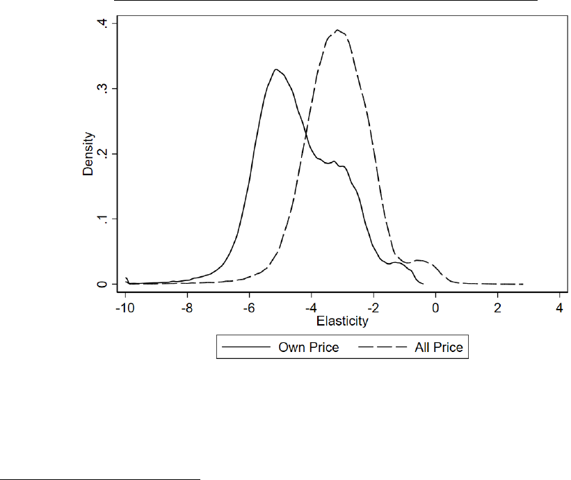
Figure 6 shows the distributions of own-price elasticity (i.e., percentage change in market share from a
percentage change in own price) and all-price elasticity (i.e., percentage change in market share from a
percentage change in price of all products). The median of the own-price elasticities is –4.41 and the median
of the all-price elasticities is –3.12.
40
Figure 7 shows average own-price elasticities for each of the 16
income groups. As expected, own-price elasticity of demand decreases with income, implying higher-
income travelers are less price sensitive.
Figure 6. Distributions of Own- and All-Price Elasticities of Demand
Notes: Own-price elasticity of demand is the percentage change in market share for a product from a 1
percent change in a product’s own price. All-price elasticity of demand is the percentage change in market
share for a product from a 1 percent change in all products’ prices. The densities are constructed using an
Epanechnikov kernel with a bandwidth of 0.05.
39
The DOT’s (2016) methodology for computing the VTTS for leisure travelers is admittedly arbitrary. Specifically,
the DOT (2016) assumes the VTTS for leisure travelers is equal to ½ hourly median income. Using high-frequency
GPS data linking drivers to their choice of gas station, Dorsey, Langer, and McRae (2022) estimate the VTTS as 89
percent of hourly median income. Using large-scale field experiments for Lyft riders, Goldszmidt et al. (2020) estimate
the VTTS as 100 percent of hourly median income. Zamparini and Reggiani (2007) report that the mean VTTS from
a meta-analysis of 90 studies was 83 percent of hourly median earnings.
40
IATA (2008) estimates an own-price elasticity of demand for short-haul, intra–North America markets as –1.65.
McWeeny (2019) finds that a model that does not account for driving time to alternative airports understates own-
price elasticities of demand by about 42 percent. Applying McWeeny’s (2019) adjustment to IATA’s (2008) estimate
would suggest an own-price elasticity of demand for short-haul, intra–North America markets of –2.87. The elasticities
I estimate are at the product level, which are expected to be larger than estimates at the market level.

25
Figure 7. Own-Price Elasticity of Demand by Income
Note: Own-price elasticity of demand is the average over all products for each of the 16 income groups
shown on the horizontal axis.
B. Model Fit and Post-Estimation Checks
Figure 8 shows the empirical distribution of driving times from the Market Locator data alongside the
model-predicted distribution of driving times. The model does a good job of fitting the data: The
distributions are similar in shape and the median driving times are very close, 33 minutes (actual) versus
36 minutes (predicted).
To assess the role of each set of moments in identifying the parameters, I compute Honoré, Jørgensen,
and de Paula’s (2020)
measure of moment informativeness, which measures the relative change in the
asymptotic variance of the estimator from the removal of a set of moments. A large relative change in the
asymptotic variance of a parameter’s estimator suggests the removed moments were informative for
identifying said parameter. I categorize the moments into five groups: (1) six interactions between four
(continuous) exogenous product characteristics (direct flight distance, extra time, origin presence, number
of daily flights) interacted with the estimated residual
; (2) squared differences from the average among
competitors for three (continuous) exogenous product characteristics (extra time, origin presence, number
of daily flights) interacted with the estimated residual
; (3) three (continuous) exogenous product
characteristics (extra time, origin presence, number of daily flights) for 11 competitors interacted with the
0
1
2
3
4
5
6
7
8
9
(–) Own
-Price Elasticity
Annual Income

26
estimated residual
; (4) the number of products in each market and share of products that are direct flights
interacted with the estimated residual
; (5) the sum over all individuals and all products of the difference
between a purchase indicator
and the model-predicted purchase probability conditional on purchase
interacted with driving time
(i.e., micromoments).
Figure 8. Actual and Predicted Distributions of Driving Times to the Airport
Sources: Airlines Reporting Corporation; Open Source Routing Machine.
Notes: Driving time is computed for a random sample of 10,000 passengers from Market Locator for
2013–19. Actual driving time comes from the data. Predicted driving time is
. The
densities are constructed using an Epanechnikov kernel with a bandwidth of 2.5 minutes.
Table 3 shows Honoré, Jørgensen, and de Paula’s (2020)
measure of moment informativeness for
the five groups of moments described above on the estimated parameters for mean price sensitivity (), the
nesting parameter (), drive time sensitivity (), and income-specific price sensitivity (
). The results
confirm the identification intuition explained in Section V.C. The most informative moments for identifying
mean and income-specific price sensitivity are those derived from Ciliberto, Murry, and Tamer’s (2021)
instruments. Identification of drive time sensitivity is driven almost entirely from the micromoments
calculated using the Market Locator data, while these micromoments have almost influence on identifying
any other parameters. Identification of the nesting parameter is driven by the moments that include the
number of products in each market as an instrument, which validates the standard practice in the literature.

27
Table 3. Moment Informativeness
Moments
Mean price
sensitivity
Nesting
parameter
Drive time
sensitivity
Income-specific
price sensitivity
1
0.595
0.522
0.054
1.537
2
0.177
0.227
0.012
0.353
3
9.584
0.629
0.053
2.680
4
2.544
2.331
0.074
0.136
5
0.000
0.024
24.630
0.000
Notes: Moment informativeness is calculated using Honoré, Jørgensen, and de
Paula’s (2020)
measure. Moments listed in the first column correspond to the five
groups explained in the text. The bolded cell in each column indicates the most
informative moment for identifying the column parameter.
VII. COUNTERFACTUAL ANALYSIS OF ESSENTIAL AIR SERVICE
In this section, I use my estimated model to perform a counterfactual policy experiment to determine
the consumer surplus that community members derive from EAS-subsidized commercial service at their
community airports. To do so, I analyze a policy environment in which all EAS subsidies are ended. As
noted in Appendix Table H3, most airports that have lost EAS eligibility no longer have commercial service,
so it is reasonable to assume that ending EAS subsidies would result in an end to commercial service.
However, it is possible that ending EAS subsidies would not end all commercial service—such as at
Hagerstown Regional Airport (HGR), which lost EAS eligibility in 2018 but still has commercial service
offered by Allegiant Air—in which case my counterfactual analysis would overestimate the value of EAS-
subsidized commercial service at an airport. Importantly, my counterfactual analysis does not assume that
all activity at the airport would be eliminated, only that subsidized commercial service would end; an airport
may provide benefits beyond commercial service—such as the ability to fly private planes into and out of
the community—and as shown in Appendix Table H3, all formerly eligible EAS airports still support
general aviation.
A. Data Construction
I use the Market Locator data to link customers’ choice of product with their home ZIP code. Generally,
when EAS community members are observed flying from an airport that is not their local airport, I assume
that they drove there. (Appendix G gives more details about the construction of the data used for the
counterfactual policy experiment.) I use the same notions of products and markets that were used in the
estimation; namely, a market is an origin region to destination airport pair, where in this case the origin
region is an EAS community. Appendix B shows constructed catchment areas for the 107 EAS airports

28
under consideration along with an array of alternative nearby airports. To avoid complications arising due
to airports changing carriers over time, I restrict my counterfactual policy analysis to using data from 2019.
At least two relevant institutional details are worth mentioning. First, EAS-eligible airports are typically
only served by one subsidized carrier at a time flying to one or two hubs.
41
,
42
Second, prices on EAS-
subsidized flights generally exhibit little to no variability within a contract period. Thus, rather than using
DB1B to compute average prices for EAS-originating flights from a sample of itineraries, I extract prices
directly from the subsidized carriers’ EAS proposals to the DOT (listed in Appendix Table H4), which
usually include the airlines’ expected average fares.
EAS community members can be thought of as having two basic choices to access commercial air
travel: via driving a short distance to their local airport for an indirect flight to their final destination, or via
driving a (potentially substantially) longer distance to an alternative airport for a direct flight to their final
destination.
43
An EAS community member’s choice set could include several nearby airports within driving
distance, such as those shown in Appendix B. I restrict the set of alternative airports to those within a 5-
hour drive from the EAS community with non-trivial market shares. Market size is assumed to be the
population of the catchment areas shown in Appendix B.
B. Methodology
The basic idea of the counterfactual policy analysis is to compare the consumer surplus that EAS
community members derive from two alternative choice sets, one that includes the option to fly on an EAS-
subsidized flight and one that does not. I calculate the change in consumer surplus from the removal of
EAS-originating products as the compensating variation using the log-sum approach (de Jong et al., 2007;
Small and Rosen, 1981). As shown by Kling and Thomson (1996), the distributional assumption on the
composite structural error term implies
41
Starting in May 2021, SkyWest, the largest regional carrier, began offering subsidized service from Yellowstone
Airport under two different brands, Delta Connection and United Express (DOT, 2021a). Previously, SkyWest only
offered service from Yellowstone Airport under the Delta Connection brand (DOT, 2019b).
42
Starting in June 2021, United Airlines offered service from Joplin Regional Airport to three hubs: O’Hare
International Airport, Denver International Airport, and George Bush Intercontinental Airport (DOT, 2021b; Joplin
Globe staff, 2021). United dropped its flight to Houston in late 2021 and filed to withdraw service at Joplin completely
in early 2022, citing pilot shortages, though the DOT ordered United to continue service at Joplin until a replacement
carrier was found (DOT, 2022a; Joplin Globe staff, 2022; Woodin, 2022).
43
For computational simplicity, I assume the driving time to the local airport for all members of an EAS community
is 0. I only consider direct flights from non-EAS airports to ensure consistent comparison of products within the
modeling framework. For example, the modeling framework does not allow for flights with more than one connection.
Only about 10 percent of EAS community members make more than one stop en route to their final destination.

29
where the sum is taken over all products
in market , excluding the outside option; and is an
unrecoverable constant.
To ascertain the consumer surplus derived from EAS-subsidized commercial service, I compute
expected consumer surplus under two choice scenarios: The true scenario where consumers have access to
all products—including those originating from EAS airports—and the counterfactual scenario where
consumers do not have access to commercial service departing from the EAS airport. Let
denote
consumer surplus from the true scenario and let
denote consumer surplus from the counterfactual
scenario. The surplus that consumer places on EAS-subsidized commercial service is the difference
between the expected value of these two quantities:
. A community’s
aggregate consumer surplus from having access to EAS-subsidized commercial service is found by
aggregating
over all community members and markets .
C. Counterfactual Results
I compute each EAS community’s aggregate expected consumer surplus from EAS-subsidized
commercial service using the above equation. As noted previously, it is plausible that removing EAS
subsidies for many EAS airports would not result in the termination of all commercial service, and might
actually result in increased service to the extent EAS subsidies act as entry barriers to competitors. Thus,
the counterfactual analysis likely overestimates the consumer surplus derived from EAS subsidies.
I find that the aggregate consumer surplus that community members derive from EAS-subsidized
commercial service at all 107 airports under consideration is about $16 million in 2019, a paltry amount
compared to EAS’s cost of roughly $290 million in 2019. From an aggregate cost–benefit perspective, it is
clear that EAS does not provide nearly enough benefits to communities to justify its costs. Figure 9 shows
the distribution of consumer surplus derived from EAS-subsidized commercial service per EAS community
member who uses the airport. On average, users of EAS airports who live in the community each derive
about $24 in consumer surplus from subsidized commercial service at the community airport, compared to
a median per-passenger subsidy of $141.
Table 4 summarizes the top 10 and bottom 10 EAS communities in terms of estimated net consumer
surplus (estimated benefits less the subsidy cost). The top 10 communities have several features in common.
First, their community airports are all among the busiest EAS airports, with 9 among the top 15 in terms of
annual enplanements. Second, they all have arguably negligible per-passenger subsidy rates, averaging less

30
than $20 per passenger, which suggests subsidies are likely not needed to sustain commercial service. Third,
they are all served by legacy carriers. Fourth, several are served by more than one airline or by one airline
but without the use of subsidies, including Grand Island, Cody, West Yellowstone, Joplin, and Sioux City.
Figure 9. Distribution of Consumer Surplus per EAS Resident User
Notes: Consumer surplus for each community is calculated using the methodology described in the text.
Consumer surplus per EAS resident user is calculated by dividing consumer surplus by the share of EAS
airport users who are deemed residents based on their home ZIP code multiplied by total enplanements at
the airport in 2019.
Anecdotal evidence suggests Joplin Regional Airport and Sioux Gateway Airport are two of the most
competitive EAS-eligible airports. From 2010 to 2018, American Airlines provided subsidized service from
Joplin to O’Hare International Airport and Dallas/Fort Worth International Airport. But not wanting to be
undercut by United—which also maintains a hub at O’Hare—American agreed to continue unsubsidized
service from 2018 to 2020, until the COVID-19 pandemic made maintaining unsubsidized service
unsustainable. American proceeded to pull out of Joplin in 2020, at which point United secured the vacated
EAS contract, agreeing to provide subsidized service from Joplin to three of its hubs: Denver International
Airport, O’Hare International Airport, and Houston George Bush Intercontinental Airport. An almost
identical story played out at Sioux Gateway Airport: From 2011 to 2016, American provided subsidized
service from Sioux City to O’Hare and Dallas/Fort Worth, but fearing competition from United, American
agreed to provide unsubsidized service from 2016 to 2020, when American pulled out due to the COVID-

31
19 pandemic and United quickly secured the EAS contract at Sioux Gateway Airport. This anecdotal
evidence is suggestive of rent-seeking behavior, as American apparently used its EAS contract at Joplin
and Sioux City to stifle competition, and United now appears to be doing the same.
Table 4. Top 10 and Bottom 10 EAS Communities Ranked by Net Consumer Surplus
Community
Airline
Price
Per-
passenger
subsidy
Total
consumer
surplus
(millions)
Total
subsidy
(millions)
Miles to
nearest
hub
Miles to
nearest
airport
Top 10 in terms of net consumer surplus
Joplin, MO
American
$102
$0.00
$0.727
$0.000
154
66
Sioux City, IA
American
$124
$0.00
$0.689
$0.000
189
89
Grand Island, NE
American
$135
$2.76
$0.469
$0.389
138
94
Cody, WY
United
$101
$10.31
$0.708
$0.850
449
107
Butte, MT
Delta
$105
$16.99
$0.336
$0.882
415
78
Garden City, KS
American
$110
$17.43
$0.291
$0.874
300
200
West Yellowstone, MT
Delta
$115
$36.14
$0.000
$0.650
332
91
Aberdeen, SD
Delta
$103
$23.50
$0.400
$1.390
270
175
Bemidji, MN
Delta
$99
$21.20
$0.257
$1.310
213
122
Pellston, MI
Delta
$96
$23.18
$0.173
$1.347
267
84
Bottom 10 in terms of net consumer surplus
Macon, GA
Contour
$89
$137.00
$0.046
$4.688
82
82
Presque Isle, ME
United
$143
$180.50
$0.260
$4.781
358
157
Page, AZ
Contour
$129
$52.90
$0.014
$4.399
282
134
Clovis, NM
Boutique
$97
$401.23
$0.035
$4.281
409
101
Sidney, MT
Cape Air
$40
$208.21
$0.052
$4.248
658
172
Greenbrier, WV
United
$79
$155.33
$0.102
$3.994
230
79
Tupelo, MS
Contour
$49
$128.74
$0.076
$3.932
94
62
Devils Lake, ND
United
$120
$284.49
$0.133
$3.935
402
84
Liberal, KS
United
$79
$174.44
$0.076
$3.748
356
176
Watertown, NY
American
$93
$87.72
$0.360
$3.950
277
66
Sources: US Department of Transportation; OpenStreetMap.
Notes: Consumer surplus for each community is calculated using the methodology described in the text.
Miles to the nearest hub is to the nearest medium or large hub. Miles to the nearest airport is miles to the
nearest commercial airport, including small hubs and non-hubs.
As additional evidence of a competitive environment, consider that 3 of the top 10 communities in
terms of net consumer surplus are served by one subsidized airline and one or more unsubsidized airlines.
Central Nebraska Regional Airport in Grand Island is served by both a subsidized airline (American
Airlines) and an unsubsidized airline (Allegiant Air), which has been providing unsubsidized service from
Grand Island to Harry Reid International Airport and Phoenix–Mesa Gateway Airport since 2008.
Yellowstone Regional Airport, located less than an hour’s drive from the east entrance of Yellowstone
32
National Park in Cody, is an attractive destination during the summer tourism season. In the summer
months, both United and Delta provide unsubsidized service to and from Yellowstone Regional Airport;
but during the non-summer months, only United provides (subsidized) service. Similarly, Yellowstone
Airport is located on the Montana–Wyoming border near the west entrance of Yellowstone National Park
and is also served by United and Delta (both subsidized), who received a waiver from the usual service
requirements in order to provide twice the number of weekly round trips during the summer months
compared to the non-summer months.
Several of the bottom 10 communities in terms of net consumer surplus (4 of the bottom 5), shown in
the bottom panel of Table 4, are served by non-legacy carriers that offer scheduled passenger service only
through EAS contracts. These non-legacy carriers typically offer much lower prices and receive much
higher per-passenger subsidies compared to the legacy carriers. Overall, prices for the non-legacy carriers
serving EAS communities average $67 one way, compared to $95 for the legacy carriers, and per-passenger
subsidies for the non-legacy carriers average $318 compared to $80 for the legacy carriers. The non-legacy
carriers tend to serve less popular routes using smaller aircraft, but the routes they serve are no more isolated
in terms of distance to the nearest medium or large hub compared to routes served by the legacy carriers.
For example, Boutique Air—whose slogan is “fly private for the cost of commercial”—offers
essentially private, EAS-subsidized flights on 9-seat Pilatus PC-12s from Cavern City Air Terminal in
Carlsbad, New Mexico, to Dallas/Fort Worth International Airport for a price of $91; yet less than 2 percent
of travelers from Carlsbad choose this option, while 36 percent choose to drive 1.25 hours to Roswell Air
Center and 23 percent choose to drive 2.75 hours to El Paso International Airport. These discrepancies
suggest there are differences in unobserved quality between legacy and non-legacy carriers such that EAS
community members would much rather drive a considerable distance to a hub than fly on a heavily
subsidized, essentially private flight from their local airport.
The bottom 10 airports in terms of net consumer surplus are also characterized by very high subsidy
rates (all exceeding $3.75 million per year) and low utilization. Prescott Regional Airport, Chippewa Valley
Regional Airport, and Middle Georgia Regional Airport are particularly egregious examples, as all three
communities are located about 90 minutes from major international airports—Phoenix Sky Harbor,
Minneapolis–Saint Paul International Airport, and Hartsfield–Jackson Atlanta International Airport,
respectively—yet only about 10 percent of travelers from Prescott choose a subsidized flight from Prescott
Regional Airport compared to 80 percent choosing to drive to Phoenix; 10 percent of travelers from Eau
Claire choose a subsidized flight from Chippewa Valley Regional Airport compared to 84 percent choosing
to drive to Minneapolis; and 3 percent of travelers from Macon choose a subsidized flight from Middle
Georgia Regional Airport compared to 94 percent choosing to drive to Atlanta. Middle Georgia Regional

33
Airport is also notable for requiring the 2nd-largest subsidy among all EAS communities, at $4.7 million
in 2019. (Appendix Figure H3 shows the distribution of annual subsidy amounts for 2019.)
D. Distributional Implications
From a distributional perspective, policymakers might be interested to know whether EAS serves those
it intends to and whether the benefits are evenly distributed among recipients. Figure 10 shows the
distribution of consumer surplus by income compared to the population distribution by income. There are
no discernable differences in the distributions, suggesting those in the community who benefit from EAS
are representative of the community as a whole in terms of income. Figure 11 shows the distribution of
consumer surplus by income for communities that are more than 210 miles from a medium or large hub
compared to communities that are less than 210 miles from a medium or large hub. Again, the distributions
are nearly identical, suggesting the distribution of consumer surplus by income is no different for
community members who live far from a hub compared to those who live close to a hub.
Figure 10. Distributions of Consumer Surplus and Population in EAS Communities by Income
Source: zip-codes.com.
Notes: Consumer surplus for each airport is calculated using the methodology described in the text.
Median household income is for the ZIP code in which the traveler resides. The distributions are smoothed
by grouping median household incomes into buckets of $5,000.
Figures 10 and 11 suggest that the benefits received by EAS community members do not differ
substantially between communities along observable characteristics. Rather, distributional discrepancies
likely arise because the main beneficiaries of the EAS programs are high-income tourists who visit the EAS
communities. While it is beyond the scope of this paper to formally estimate the consumer surplus that

34
tourists derive from EAS, back-of-the-envelope calculations can provide a sense of how much tourism is
potentially generated by an EAS airport and its contribution to the local economy. Although it is not the
statutory purpose of EAS to promote local tourism, policymakers representing districts with EAS-
subsidized service often brag about the impact that the program has on their local economies.
44
Figure 11. Distributions of Consumer Surplus in EAS Communities by Income and Distance from Hub
Source: zip-codes.com.
Notes: Consumer surplus for each community is calculated using the methodology described in the text.
The solid line is for EAS communities located less than 210 miles from a medium or large hub. The dashed
line is for EAS communities located more than 210 miles from a medium or large hub. Median household
income is for the ZIP code in which the traveler resides. The distributions are smoothed by grouping median
household incomes into buckets of $5,000.
Appendix Table H2 shows 21 EAS airports that serve as gateways to 23 national parks. The table shows
total annual visitors to the parks along with the total number of nonresidents using the nearby EAS airport.
In every case, the number of visitors flying into the EAS airport is trivial compared to the parks’ total annual
visitors, suggesting a vast majority of visitors arrive at the parks by driving. Thus, even if the EAS
communities nearby national parks were to lose subsidies and lose commercial service, the effect on
regional tourism would likely be trivial.
Figure 12 shows the change in the distribution of driving time from the removal of the EAS option,
shown separately for communities located less than 210 miles from a hub and communities located more
than 210 miles from a hub. The median of the actual distribution of driving time 116 minutes. The
44
Elise Stefanik, for example, who in 2021 represented five EAS communities in upstate New York, boasts that EAS
“attracts travelers to our region, while boosting small businesses and tourist areas” (Stefanik, 2021).

35
counterfactual distributions of driving time are constructed by removing products originating at EAS-
subsidized airports from community members’ choice sets.
45
The counterfactual distribution of driving time
is clearly bimodal: The median of the distribution for communities located less than 210 miles from a hub
is 168 minutes and the median of the distribution for communities located more than 210 miles from a hub
is 297 minutes. The bimodal nature of the counterfactual distribution suggests that, even though isolated
communities have alternative options (see Figure 2 and Appendix B), these alternative airports are less
accessible or less attractive compared to alternative airports nearby less isolated communities.
Figure 12. Actual and Counterfactual Distributions of Driving Time for EAS Communities
Sources: Federal Aviation Administration; Airlines Reporting Corporation; OpenStreetMap.
Notes: The distributions are constructed by taking the average driving time weighted by product shares
for each of the 107 EAS communities. The counterfactual distributions are constructed by removing
products originating from EAS-subsidized airports. Counterfactual distributions are shown separately for
EAS communities located less than and more than 210 miles from a medium or large hub. The densities
are constructed using an Epanechnikov kernel with a bandwidth of 20 minutes.
45
The distributions are constructed conditional on flying. The model predicts that about 20 percent of passengers
switched to an alternative product under the counterfactual scenario while about 80 percent switched to the outside
option.

36
VIII. CONCLUSIONS
The aviation industry has completely transformed in the almost half century after the great airline
deregulation experiment. Yet despite the major changes to passenger aviation around the country, Essential
Air Service, a remnant of the pre-deregulation era designed to be temporary and transitional, has persisted.
46
I have presented evidence in this paper that suggests EAS is a regressive program that provides very little
value to the communities it is meant to serve.
Several broad conclusions can be drawn from the counterfactual policy analysis. First, the costs of
maintaining subsidized service at all EAS-eligible communities are considerably higher than the benefits
residents derive: In aggregate, the EAS program cost $290 million in 2019 yet EAS community members
received only $16 million in consumer surplus. Second, there were no discernable differences in the
distributions of consumer surplus among EAS communities by income or distance to the nearest hub,
suggesting EAS does not disproportionately benefit high-income people within EAS communities. Third,
airports that provide the largest benefits to EAS communities are primarily served by legacy airlines with
per-passenger subsidy rates so low as to be negligible, while airports that provide the lowest benefits to
EAS communities are served by a mixture of legacy and non-legacy carriers that require high per-passenger
subsidies. Fourth, EAS airports that provide the most benefit to their communities tend to have features of
a competitive environment, such as competition between multiple airlines and legacy carriers providing
unsubsidized service in order to keep competitors out.
At least two novel insights can be drawn from simple tabulations of the proprietary Market Locator
data linking airline passenger purchases to their home ZIP code. First, travelers in nearly every EAS
community not only have other options available to them when it comes to accessing commercial air travel,
they also prefer those options—with many choosing to drive several hours to a larger airport rather than to
take a subsidized flight from their local airport—although communities located farther from a medium or
large hub face greater barriers to accessing commercial air travel. Second, EAS community members are
not the primary users of EAS airports nor the main beneficiaries of EAS subsidies, as tourists and other
visitors make up 57 percent EAS airport users and have about 18 percent higher incomes than residents on
average. Thus, EAS does a poor job of targeting its intended beneficiaries (i.e., members of the community),
and instead serves to subsidize well-off outsiders to visit national parks and other points of interest where
EAS communities happen to be located.
46
EAS is a classic example of a government program with concentrated benefits and diffuse costs, which may explain
why EAS has continued to persist. Hall, Ross, and Yencha (2015) find that higher EAS subsidies are associated with
airports located in districts with congressional representatives on the Transportation Committee, which handle renewal
of the EAS program, and the Ways and Means Committee, which has jurisdiction over the Airport and Airway Trust
Fund from which EAS is funded. Appendix Figure H2 shows the political leanings of EAS communities based on the
Cook Political Report’s Partisan Voting Index.
37
While this paper provides novel insights into the airline industry, it is not without its limitations. First,
I only considered the implications of airport substitution on demand. Jointly estimating a model of supply
could provide a fuller picture of the implications of rent-seeking and airport substitution, particularly as it
relates to antitrust and merger analyses. Future work should investigate the implications of airport
substitution and market definition for merger analyses. Second, I assumed airlines’ network structures were
exogenous with respect to product-level unobserved quality, though recent work by Ciliberto, Murry, and
Tamer (2021) has attempted to relax this assumption. Third, I only considered the benefit of EAS to
members of EAS-eligible communities and did not formally model the choice behavior or quantify the
benefit of EAS to travelers living outside of EAS communities.
Policymakers should consider whether Essential Air Service is still essential in the 21st century. The
airline industry has dramatically changed since deregulation in 1978, and the EAS program has not evolved
with the times. Congress could continue to limit the scope of the program by enacting more stringent
eligibility requirements. Two simple reforms Congress could enact would be to include distance to small
hubs in addition to medium and large hubs when determining EAS eligibility, and to increase the minimum
allowable distance to a hub beyond 70 miles. Such reforms would do a better job of targeting communities
that actually face significant barriers to commercial air travel. Eliminating EAS entirely has the potential
to benefit the communities it is meant to serve and would move the US closer to realizing the full societal
benefits of airline deregulation.
ACKNOWLEDGMENTS
I am grateful for many helpful comments received from Gaurab Aryal, Lane Cohee, Kristina Currans,
Gautam Gowrisankaran, Daniel Herbst, Ashley Langer, Dennis McWeeny, Juan Pantano, Stanley
Reynolds, Mark Stegeman, Matthijs Wildenbeest, Clifford Winston, and Mo Xiao. I thank Chris Conlon,
Jeff Gortmaker, and Juan Velez for sharing code and advice. Lastly, I thank Devon Barnett, John Heimlich,
Kenneth Strickland, and Daniel Swain for helpful discussions and for providing access to data. High
Performance Computing resources were provided by the Research Data Center at the University of Arizona.
Funding was provided by the National Institute for Transportation and Communities, the Graduate and
Professional Student Council at the University of Arizona, and the Department of Economics at the
University of Arizona.
38
REFERENCES
Adler, Thomas, C. Stacey Falzarano, and Gregory Spitz. 2005. “Modeling Service Trade-Offs in Air
Itinerary Choices.” Transportation Research Record, no. 1915: 20–26.
Bao, Ken, Abby Wood, and Ray A. Mundy. 2015. “Cost–Benefit Analysis: Substituting Ground
Transportation for Subsidized Essential Air Service.” University of Missouri–St. Louis, Center for
Transportation Studies.
Berry, Steven T. 1990. “Airport Presence as Product Differentiation.” American Economic Review 80, no.
2: 394–99.
———. 1994. “Estimating Discrete-Choice Models of Product Differentiation.” RAND Journal of
Economics 25, no. 2: 242–62.
Berry, Steven, Michael Carnall, and Pablo T. Spiller. 1996. “Airline Hubs, Markups and the Implications
of Customer Heterogeneity.” Working Paper no. 5561. National Bureau of Economic Research.
———. 2006. “Airline Hubs: Costs, Markups and the Implications of Customer Heterogeneity.” In
Advances in Airline Economics, Volume 1: Competition Policy and Antitrust, edited by Darin Lee.
Emerald.
Berry, Steven, and Panle Jia. 2010. “Tracing the Woes: An Empirical Analysis of the Airline Industry.”
American Economic Journal: Microeconomics 2, no. 3: 1–43.
Berry, Steven, James Levinsohn, and Ariel Pakes. 1995. “Automobile Prices in Market Equilibrium.”
Econometrica 63, no. 4: 841–90.
———. 2004. “Differentiated Products Demand Systems from a Combination of Micro and Macro Data:
The New Car Market.” Journal of Political Economy 112, no. 1: 68–105.
Borenstein, Severin. 1989. “Hubs and High Fares: Dominance and Market Power in the U.S. Airline
Industry.” RAND Journal of Economics 20, no. 3: 344–65.
Brueckner, Jan K., Darin Lee, and Ethan Singer. 2014. “City-Pairs versus Airport-Pairs: A Market-
Definition Methodology for the Airline Industry.” Review of Industrial Organization 44, no. 1: 1–25.
Cape Air. 2018. “Cape Air’s Decatur Service Set to Start February 14, 2018.” Press Release, January 12.
https://www.capeair.com/theme/single-news.html?id=1394
Cardell, N. Scott. 1997. “Variance Components Structures for the Extreme-Value and Logistic
Distributions with Application to Models of Heterogeneity.” Econometric Theory 13, no. 2: 185–213.
Ciliberto, Federico, Charles Murry, and Elie Tamer. 2021. “Market Structure and Competition in Airline
Markets.” Journal of Political Economy 129, no. 11: 2995–3038.
Ciliberto, Federico, and Jonathan W. Williams. 2014. “Does Multimarket Contact Facilitate Tacit
Collusion? Inference on Conduct Parameters in the Airline Industry.” RAND Journal of Economics 45,
no. 4: 764–91.
39
Conlon, Christopher, and Jeff Gortmaker. 2020. “Best Practices for Differentiated Products Demand
Estimation with PyBLP.” RAND Journal of Economics 51, no. 4: 1108–61.
Cunningham, Lawrence F., and E. Woodrow Eckard. 1987. “U.S. Small Community Air Service Subsidies:
Essential or Superfluous?” Journal of Transport Economics and Policy 21, no. 3: 255–77.
Daly, Andrew, Flavia Tsang, and Charlene Rohr. 2014. “The Value of Small Time Savings for Non-
Business Travel.” Journal of Transport Economics and Policy 48, no. 2: 205–18.
Davis, Peter. 2006. “Spatial Competition in Retail Markets: Movie Theaters.” RAND Journal of Economics
37, no. 4: 964–82.
de Jong, Gerard, Andrew Daly, Marits Pieters, and Toon van der Hoorn. 2007. “The Logsum as an
Evaluation Measure: Review of the Literature and New Results.” Transportation Research Part A:
Policy and Practice 41, no. 9: 874–89.
de Neufville, Richard. 1995. “Management of Multi-Airport Systems: A Development Strategy.” Journal
of Air Transport Management 2, no. 2: 99–110.
Dorsey, Jackson, Ashley Langer, and Shaun McRae. 2022. “Fueling Alternatives: Gas Station Choice and
the Implications for Electric Charging.” Working Paper no. 29831. National Bureau of Economic
Research.
Drukker, Austin J., and Clifford Winston. Forthcoming. “Public Airport Competition and Some Potential
Benefits of Private Airport Competition.” In Revitalizing a Nation: Competition and Innovation in the
US Transportation System, edited by Clifford Winston and Jia Yan. Brookings Institution Press.
Eno Center for Transportation. 2018. “Question: How Does the Federal Government Subsidize Air Service
to Small Communities?” Aviation Insights, no. 10.
Evans, William N., and Ioannis N. Kessides. 1993. “Localized Market Power in the U.S. Airline Industry.”
Review of Economics and Statistics 75, no. 1: 66–75.
Federal Aviation Administration (FAA). 2020. “The Economic Impact of Civil Aviation on the U.S.
Economy.” https://www.faa.gov/about/plans_reports/media/2020_jan_economic_impact_report.pdf
———. 2022. “Air Traffic by the Numbers.” https://www.faa.gov/sites/faa.gov/files/air_traffic/
by_the_numbers/Air_Traffic_by_the_Numbers_2022.pdf
Fournier, Gary M., Monica E. Hartmann, and Thomas W. Zuehlke. 2007. “Airport Substitution by
Travelers: Why Do We Have to Drive to Fly?” In Advances in Airline Economics, Volume 2: The
Economics of Airline Institutions, Operations and Marketing, edited by Darin Lee. Emerald.
Goldszmidt, Ariel, John A. List, Robert D. Metcalfe, Ian Muir, V. Kerry Smith, and Jenny Wang. 2020.
“The Value of Time in the United States: Estimates from Nationwide Natural Field Experiments.”
Working Paper no. 28208. National Bureau of Economic Research.
40
Grigolon, Laura, and Frank Verboven. 2014. “Nested Logit or Random Coefficients Logit? A Comparison
of Alternative Discrete Choice Models of Product Differentiation.” Review of Economics and Statistics
96, no. 5: 916–35.
Grubesic, Tony H., and Timothy C. Matisziw. 2011. “A Spatial Analysis of Air Transport Access and the
Essential Air Service Program in the United States.” Journal of Transport Geography 19, no. 1: 93–
105.
Grubesic, Tony H., and Fangwu Wei. 2013. “Essential Air Service: A Local, Geographic Market
Perspective.” Journal of Transport Geography 30: 17–25.
Hall, Joshua, Amanda Ross, and Christopher Yencha. 2015. “The Political Economy of the Essential Air
Service Program.” Public Choice 165, nos. 1–2: 147–64.
Hansen, Lars Peter. 1982. “Large Sample Properties of Generalized Method of Moments Estimators.”
Econometrica 50, no. 4: 1029–54.
Hatfield, John William, and Jonathan Wallen. 2022. “Many Markets Make Good Neighbors: Multimarket
Contact and Deposit Banking.” Working paper. https://www.hbs.edu/faculty/Pages/item.aspx?num=
61741
Hess, Stephane, Thomas Adler, and John W. Polak. 2007. “Modelling Airport and Airline Choice
Behaviour with the Use of Stated Preference Survey Data.” Transportation Research Part E: Logistics
and Transportation Review 43, no. 3: 221–33.
Hess, Stephane, and John W. Polak. 2005. “Mixed Logit Modelling of Airport Choice in Multi-Airport
Regions.” Journal of Air Transport Management 11, no. 2: 59–68.
———. 2006. “Airport, Airline and Access Mode Choice in the San Francisco Bay Area.” Papers in
Regional Science 85, no. 4: 543–67.
Ho, Katherine, and Joy Ishii. 2011. “Location and Competition in Retail Banking.” International Journal
of Industrial Organization 29, no. 5: 537–46.
Honoré, Bo, Thomas Jørgensen, and Áureo de Paula. 2020. “The Informativeness of Estimation Moments.”
Journal of Applied Econometrics 35, no. 7: 797–813.
International Air Transport Association (IATA). “Air Travel Demand.” Economics Briefing no. 9.
https://www.iata.org/en/iata-repository/publications/economic-reports/air-travel-demand/
———. 2019. “The Value of Air Transport in the United States.”
https://www.iata.org/contentassets/cf15de08044e49b6b6e1ebf8a3513ed4/economic-studies-usa-eng-
final.pdf
Ishii, Jun, Sunyoung Jun, and Kurt Van Dender. 2007. “Assessing the Role of Airlines and Airports in
Multi-Airport Markets.” In Advances in Airline Economics, Volume 2: The Economics of Airline
Institutions, Operations and Marketing, edited by Darin Lee. Emerald.
41
———. 2009. “Air Travel Choices in Multi-Airport Markets.” Journal of Urban Economics 65: 216–27.
Joplin Globe staff. 2021. “Joplin Adds Houston as Third Flight Hub.” Joplin Globe, March 30.
———. 2022. “SkyWest to End Air Service at Joplin Airport.” Joplin Globe, March 11.
Katz, Michael. 2007. “Estimating Supermarket Choice Using Moment Inequalities.” Job Market Paper,
Harvard University. https://www.proquest.com/docview/304849069/BEC1AF13C1F2416CPQ/1
Kling, Catherine L., and Cynthia J. Thomson. 1996. “The Implications of Model Specification for Welfare
Estimation in Nested Logit Models.” American Journal of Agricultural Economics 78, no. 1: 103–14.
Landau, Steven, Geoffrey D. Gosling, Kenneth Small, and Thomas Adler. 2016. “Measuring Air Carrier
Passengers’ Values of Time by Trip Component.” Transportation Research Record, no. 2569: 24–31.
Lowell, Dana, Tom Curry, Lily Hoffman-Andrews, and Lea Reynolds. 2011. “Comparison of Essential Air
Service Program to Alternative Coach Bus Service: Keeping Rural Communities Connected.” M. J.
Bradley & Associates.
Mahoney, Dan, and Wesley W. Wilson. 2014. “Airport and Airline Substitution Effects in Multi-Airport
Markets.” In Advances in Airline Economics, Volume 4: The Economics of International Airline
Transport, edited by James Peoples. Emerald.
Manuszak, Mark D., and Charles C. Moul. 2009. “How Far for a Buck? Tax Differences and the Location
of Retail Gasoline Activity in Southeast Chicagoland.” Review of Economics and Statistics 91, no. 4:
744–65.
McWeeny, Dennis B. 2019. “Spatial Competition in the Airline Industry.” Job Market Paper, University of
Wisconsin. https://ssrn.com/abstract=3465104
Merkert, Rico, and Matthew Beck. 2017. “Value of Travel Time Savings and Willingness to Pay for
Regional Aviation.” Transportation Research Part A: Policy and Practice 96: 29–42.
Morrison, Steven, and Clifford Winston. 1986. The Economic Effects of Airline Deregulation. Brookings
Institution Press.
———. 1989. “Enhancing the Performance of the Deregulated Air Transportation System.” Brookings
Papers on Economics Activity: Microeconomics 1, no. 1: 61–112.
Murry, Charles. 2017. “Advertising in Vertical Relationships: An Equilibrium Model of the Automobile
Industry.” Job Market Paper, Pennsylvania State University. https://ssrn.com/abstract=2549247
Murry, Charles, and Yiyi Zhou. 2020. “Consumer Search and Automobile Dealer Colocation.”
Management Science 66, no. 5: 1909–34.
Petrin, Amil. 2002. “Quantifying the Benefits of New Products: The Case of the Minivan.” Journal of
Political Economy 110, no. 4: 705–29.
Small, Kenneth A., and Harvey S. Rosen. 1981. “Applied Welfare Economics with Discrete Choice
Models.” Econometrica 49, no. 1: 105–30.
42
Smith, Howard. 2004. “Supermarket Choice and Supermarket Competition in Market Equilibrium.” Review
of Economic Studies 71, no. 1: 235–63.
Stefanik, Elise. 2021. “Stefanik Announces SkyWest to Continue Essential Air Service into Ogdensburg.”
Press Release, March 1. https://stefanik.house.gov/2021/3/stefanik-announces-skywest-continue-
essential-air-service-ogdensburg
Tang, Rachel Y. 2018. “Essential Air Service (EAS).” Report no. 44176. Congressional Research Service.
US Department of Transportation (DOT). 2016. “The Value of Time Savings: Departmental Guidance for
Conducting Economic Evaluations.” https://www.transportation.gov/office-policy/transportation-
policy/revised-departmental-guidance-valuation-travel-time-economic
———. 2017. “Order Selecting Airlines and Establishing Annual Subsidy Rates.” DOT-OST-2006-23929-
0075 (Order 2017-12-20). https://www.regulations.gov/document/DOT-OST-2006-23929-0075
———. 2019a. “$200 Per Passenger Compliance Status Report – 12 Months Ended September 30, 2019.”
https://www.transportation.gov/EAS_%24200_Per_Pax_Cap_Sep_30_2019
———. 2019b. “Order Re-Selecting Air Carrier.” DOT-OST-2003-14626-0069 (Order 2019-3-4).
https://www.regulations.gov/document/DOT-OST-2003-14626-0069
———. 2021a. “Order Selecting Air Carrier.” DOT-OST-2003-14626 (Order 2021-3-20).
https://www.regulations.gov/document/DOT-OST-2003-14626-0086
———. 2021b. “Order Selecting Air Carrier and Setting Rates for Hold-In Period.” DOT-OST-2006-
23932-0091 (Order 2021-3-2). https://www.regulations.gov/document/DOT-OST-2006-23932-0091
———. 2021c. “Subsidized Essential Air Service Communities and Distances to Nearest Hubs.”
https://www.transportation.gov/office-policy/aviation-policy/subsidized-essential-air-service-
communities-and-distances-nearest
———. 2022a. “Order Prohibiting Termination of Service and Requesting Proposals.” DOT-OST-2006-
23932-0097 (Order 2022-3-8). https://www.regulations.gov/document/DOT-OST-2006-23932-0097
———. 2022b. “Subsidized Essential Air Service Communities (48 Contiguous States, Hawaii, and Puerto
Rico).” https://www.transportation.gov/Subsidized_EAS_report48states_HI_PR_Jun2022
Woodin, Debby. 2022. “SkyWest Flights to Continue for the Year.” Joplin Globe, June 29.
Yirgu, Kaleab Woldeyohannes, and Amy M. Kim. 2021. “Aviation Fuel and Emissions in Air Markets with
Interregional Passenger Leakage.” Transportation Research Part D: Transport and Environment 101:
article 103092.
Yirgu, Kaleab Woldeyohannes, Amy M. Kim, and Megan S. Ryerson. 2021. “Long-Distance Airport
Substitution and Air Market Leakage: Empirical Investigations in the U.S. Midwest.” Transportation
Research Record 2675, no. 10: 148–60.
43
Zamparini, Luca, and Aura Reggiani. 2007. “Meta-Analysis and the Value of Travel Time Savings: A
Transatlantic Perspective in Passenger Transport.” Networks and Spatial Economics 7, no. 4: 377–96.

44
Appendix A. Catchment Areas and Population Densities for Estimation Regions
Appendix Figure A1. Estimation Regions and Airports on One Map
Source: zip-codes.com.
Notes: Each colored area represents an origin region, each geographical unit within the regions represents
a ZIP code, and darker shading represents higher population density. The dots represent airports that serve
residents of the regions.

45
Appendix Figure A2. Estimation Regions and Airports Separated by Region
Atlanta Austin Boston
Charlotte Chicago Cincinnati

46
Cleveland Columbus Dallas
Denver Detroit Fort Myers
Hartford Houston Indianapolis
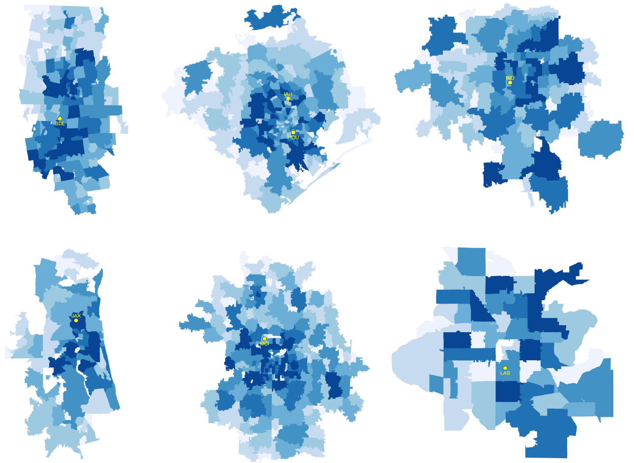
47
Jacksonville Kansas City Las Vegas
Los Angeles Miami Milwaukee Minneapolis

48
Nashville New Orleans New York
Orlando Philadelphia Phoenix

49
Pittsburgh Portland Raleigh/Durham
Sacramento Salt Lake City San Antonio

50
San Diego San Francisco Seattle
St. Louis Tampa Washington

51
Source: zip-codes.com.
Notes: Each panel represents an origin region, each geographical unit within the regions represents a ZIP code, and darker shading represents higher population
density. The dots represent airports that serve residents of the regions.

52
Appendix B. Catchment Areas, Population Densities, and Nearby Airports for EAS Regions
Alabama / Mississippi Arizona Arkansas
California Colorado Georgia
Illinois Iowa Kansas

53
Kentucky / Tennessee Maine Michigan / Wisconsin
Minnesota Missouri Montana / Wyoming

54
Nebraska New Hampshire / Vermont New Mexico
New York North Dakota / South Dakota Oregon

55
Pennsylvania Texas Utah

56
Virginia / West Virginia
Sources: Airlines Reporting Corporation; zip-codes.com.
Notes: Each panel shows a cluster of EAS communities, which are made up of ZIP codes, where darker shading
corresponds to higher population density. The yellow dots are airports receiving EAS-subsidized service. The orange dots
are a sampling of airports used by residents of the EAS communities shown in each panel.
57
Appendix C. Legal Statutes Governing EAS Eligibility
See Tang (2018) for a primer on the EAS program, its legal history, and eligibility rules. EAS typically
subsidizes one airline to provide two to four round trips per day, six days per week, from an EAS community
to a larger hub, as codified by 49 U.S.C. § 41732. Since the passage of the FAA Modernization and Reform
Act in 2012, except for Alaska and Hawaii, communities are only eligible for EAS if they received subsidies
in fiscal year 2011, and no new communities can enter the program even if they were formerly eligible.
The Related Agencies Appropriations Act of 2000 prohibits subsidies to carriers for service provided
to communities located fewer than 70 miles from the nearest medium or large hub airport. A large hub
receives more than 1 percent of annual commercial enplanements (approximately 10 million or more
passenger boardings per year), a medium hub receives between 0.25 and 1 percent of total enplanements
(approximately 3 million or more passenger boardings per year), a small hub receives between 0.05 and
0.25 percent of total commercial enplanements (approximately 500,000 or more passenger boardings per
year), and a non-hub primary airport receives between 10,000 passengers and 0.05 percent of total
commercial enplanements. The Consolidated Appropriations Act of 2014, Continued Appropriations
Resolution of 2015, and Consolidated Appropriations Act of 2018 require EAS airports located less than
40 miles from a small hub to have a cost-sharing agreement with the DOT. Hub classification can change
each year based on changing passenger volumes; see DOT (2021). Although EAS eligibility is based on a
community’s distance to the nearest medium or large hub, airlines that receive EAS contracts are not
required to fly passengers to the nearest hub nor to a medium or large hub.
According to the DOT (2014), its longstanding practice is to measure distance to a hub as the shortest
driving distance from the “center of the EAS community” to the “entrance of the nearest large or medium
hub airport” as determined by the Federal Highway Administration. More precisely, according to Grubesic
and Matisziw (2011), based on phone conversations with the DOT, distance to a hub is typically measured
from the location of a community’s city hall to the property boundary of an airport using the shortest
network path. The Vision 100—Century of Aviation Reauthorization Act of 2003 directs the DOT to
consult with state governors to determine the “most commonly used route” between the community and the
nearest large or medium hub to establish eligibility.
The Related Agencies Appropriations Act of 2000 prohibits EAS for communities that require a per-
passenger subsidy rate in excess of $200, unless the community is located more than 210 miles from the
nearest large or medium hub; and the Airport and Airway Extension Act of 2011 prohibits EAS for
communities that require per-passenger subsidy rates in excess of $1,000, regardless of distance from the
nearest hub. Subsidy cutoffs are calculated by dividing the annual subsidy by the annual passengers
generated (outbound plus inbound), and compliance is evaluated at the end of each fiscal year; see DOT
(2019). The FAA Modernization and Reform Act of 2012 requires carriers serving EAS communities to
58
maintain an average of 10 or more enplanements per day, but also gives the DOT discretion to grant
temporary waivers to communities that do not meet the per-passenger subsidy or daily enplanements rules;
see DOT (2014).
Airlines compete for EAS contracts through a bidding process, and the DOT typically receives 1–3
proposals per airport every 1–3 years, when EAS contracts typically expire. By law, the DOT must take
into account the views of the community when deciding which proposal to accept, as well as the carrier’s
service reliability and any arrangements it has with larger carriers at the hub. Notably, subsidy cost is not
among the factors the DOT is required by law to consider when evaluating bids, and if more than one carrier
proposes to offer service then local officials are under no obligation to favor the proposal that entails the
lowest cost to the federal government. 49 U.S.C. 41733(c)(1) states that the DOT shall consider the
following five factors when making a carrier selection: (1) demonstrated reliability of the carrier in
providing scheduled air service, (2) contractual and marketing arrangements the carrier has with a larger
carrier at the hub, (3) interline agreements that the carrier has with a larger carrier at the hub, (4) preferences
of the community, and (5) how the carrier proposes to market the service to members of the community.
49 U.S.C. 41733(c)(1)(D) instructs the DOT to give “substantial weight” to the views of the community.
The Consolidated and Further Continuing Appropriations Act of 2015 (Pub. L. 113-235, 128 Stat. 2699)
and subsequent Consolidated Appropriations Acts (Pub. L. 114-113, 129 Stat. 2837; Pub. L. 116-260, 134
Stat. 1827) state that the DOT may consider the relative subsidy requirements of the carriers when making
a carrier selection, and the DOT has on occasion exercised this prerogative.
59
Appendix D. Value of Travel Time Savings Using Official DOT (2016) Methodology
Business Travelers
The calculation of the value of travel time savings (VTTS) for business travelers using the DOT’s
(2016) methodology with data from 2019 is as follows: The DOT (2016, p. 8) notes that “there is wide
agreement that the VTTS for business travel should equal the gross hourly cost of employment, including
payroll taxes and fringe benefits.” According to the US Bureau of Labor Statistics’ quarterly reports on
employer costs for employee compensation (www.bls.gov/ect), average employee compensation was
roughly $35 per hour in 2019. To adjust for the higher incomes of business air travelers compared to the
median household, this value is multiplied by 2.5, which is the ratio of median household income for
business air travelers from the National Household Travel Survey to the median household income from
the US Census Bureau. So the VTTS for business air travelers is $87.50 (= $35 × 2.5) per hour.
Leisure Travelers
The calculation of VTTS for leisure travelers using the DOT’s (2016) methodology with data from
2019 is as follows: The DOT (2016, p. 5) notes that “leisure time is seen … as an object of consumption
that can be substituted for other desirable objects according to individual preferences,” hence “VTTS is
estimated to be lower for personal than for business travel” (Mackie, Jara-Díaz, and Fowkes, 2001). Noting
“the absence of a theoretically compelling hypothesis” (DOT, 2016, p. 8), for local personal travel, “VTTS
is estimated at 50 percent of hourly median household income” (p. 11), following Small (1992); however,
since “research has found evidence of a moderate rise in VTTS with trip distance” (p. 7), the DOT (2016)
applies “a ratio of VTTS to hourly income of 70 percent” (p. 11), or a 20 percent premium. According to
the US Census Bureau, median household income in 2019 was $68,700. Dividing by 2,080 (= 40 × 52)
annual working hours yields income of $33 per hour. To adjust for the higher incomes of air travelers
compared to the median household, this value is multiplied by 1.9, which is the ratio of median household
income for leisure air travelers from the National Household Travel Survey to the median household income
from the US Census Bureau. So the VTTS for leisure travelers is $44 (= $33 × 1.9 × [0.5 + 0.2]) per hour.
Assuming VTTS is 100 percent of hourly median earnings, following Goldszmidt et al. (2020), the VTTS
for leisure travelers is $75 (= $33 × 1.9 × [1 + 0.2]).

60
Appendix E. Construction of Income Distributions at the ZIP Code Level
Income distributions at the ZIP code level were constructed by building up from smaller geographic
entities, specifically, Census block groups, following a procedure similar to Langer and Lemoine (2022).
Appendix Figure E1 shows the US Census Bureau’s standard hierarchy of Census geographic entities. The
smallest geographic entity at which the Census Bureau publicly releases income information is the block
group level. I am interested in constructing income distributions at the ZIP code level—or ZIP Code
Tabulation Area (ZCTA), the Census Bureau’s equivalent to the US Postal Service concept—which do not
perfectly nest with block groups. In other words, ZCTAs can overlap multiple block groups and vice versa.
Appendix Figure E1. Standard Hierarchy of Census Geographic Entities
Source: US Census Bureau.
Note: Lines connect entities that perfectly nest.
The American Community Survey (ACS) contains information about the number of households living
in each Census block group with income in each of 16 income buckets ranging from $0 to $200,000 and
above. The 16 income buckets are: $0–$10,000; $10,000–$15,000; $15,000–$20,000; $20,000–$25,000;
$25,000–$30,000; $30,000–$35,000; $35,000–$40,000; $40,000–$45,000; $45,000–$50,000; $50,000–
61
$60,000; $60,000–$75,000; $75,000–$100,000; $100,000–$125,000; $125,000–$150,000; $150,000–
$200,000; $200,000 and above.
A block group to ZCTA crosswalk was obtained from the Missouri Census Data Center. The crosswalk,
which provides the share of the population of each block group that lives in each ZCTA, was used to allocate
the number of households in each block group into each ZCTA. (This allocation implicitly assumes a
uniform distribution of households by income within block groups.) Once block group populations are
allocated to ZCTAs, the total number of households in each ZCTA and income bucket are computed. These
ZCTA and income bucket pairs are known as “cells” and are denoted by the subscript in the model
exposition. Finally, the number of households in each ZCTA and income bucket are converted to population
shares by dividing by the total population of the origin region (see Appendix Table H1). These shares are
referred to as “population weights”
in Appendix F. For each region (see Appendix A), the total number
of cells is equal to 16 times the number of ZCTAs in the region. Purchase probabilities for each product
are computed for each cell , and market shares for product are computed by aggregating over cells in a
region using population weights
(see Appendix F).

62
Appendix F. Estimation and Computational Details
Market Shares
Utility for individual from purchasing product from market is
where
The composite error term
follows the necessary distribution to generate the nested
logit model (Cardell, 1997). As shown by Berry (1994) and others, the probability that individual
purchases product from market can be written
where
is the inclusive value of the airline product nest, with the summation taken over all airline products
in
market .
Market shares for product are found by aggregating purchase probabilities over all the individuals in
a market:
where
is the population weight of each individual. For each origin region,
is equal to the number of
households in an income bucket living in a ZIP code as a share of the total origin region population (see
Appendix E), so the weights
sum to 1 for each region.
Contraction Mapping
Equate the model-predicted market shares
to the observed market shares
,
, where
,
, and
. As shown by Berry, Gandhi, and

63
Haile (2013), if
for all
and for all then there is at most one that satisfies
the above equation, which is found by inverting the equation such that
. To compute for a
given value of the parameters
, Grigolon and Verboven (2014) show that the modified mapping of Berry,
Levinsohn, and Pakes (1995),
is a contraction for the nested logit model, so by the contraction mapping theorem there exists a unique
fixed point
such that
. As shown by Berry and Haile (2014), normalizing
implies
is identified for all products and for all markets.
A consistent estimator of
is obtained by estimating the mean utility equation
via two-stage least squares, where
is an element of the fixed point described above. The residual
is a consistent estimator of
, where
is the two-stage least squares
estimator.
Macromoments
Let
be the set of exogenous instruments. The moment conditions are
. Since
then by the law of large numbers
where the summation is taken over all products and markets. Define
and the moment
where the summation is taken over all products and all markets. Note that the dimension of
is
. The moment condition is satisfied because
.
Micromoments
Let
if individual purchased product in market and
otherwise. Let
denote the
probability that individual purchases product in market conditional on purchasing an airline product:

64
where
refers to all products in market , including product , but excluding the outside option. The
moment conditions are
, where the expectation is taken over individuals and
products within a market. Define
and the moment
where the summation is taken over all individuals, products, and markets. Note that the dimension of
is . The moment condition is satisfied because
.
Efficient GMM Estimation and Standard Errors
To estimate the parameters
, stack the moments
and
to form
Note that the dimension of
is
and that
, satisfying the moment condition.
Form the objective function as
where is a
matrix that assigns weights to the moments. The estimator
searches
for parameter values that minimize the objective function up to some convergence tolerance:
An efficient estimator of the parameters is found by using the optimal weight matrix
, where
and
The weight matrix
is optimal because it assigns more weight to more precisely estimated
moments. Since
is unknown, it is infeasible to compute , so I employ the two-step procedure described
by Hansen (1982) to construct a consistent estimator of
to use as the weight matrix. As noted by Petrin
(2002), since the two sources of variance in
come from independent sampling processes, the optimal
weight matrix is block-diagonal, with an upper block of dimension corresponding to
and a
lower block of dimension corresponding to
. In the first step, a consistent estimator
is found
by setting the upper block equal to
, where
, and the lower block equal to the

65
identity matrix. In the second step, I obtain an efficient estimator
using the following weight matrix in
the second step:
where
and
. I estimate the upper block as
where the summation is taken over all products and markets and
is a diagonal matrix with squared
residuals
on the diagonal. I estimate the lower block as:
where the summation is taken over all individuals, products, and markets. Note that
so
is a
consistent estimator of the optimal weight matrix.
Standard errors are computed numerically using the expressions for asymptotic variance from Hansen
(1982), Berry, Levinsohn, and Pakes (1995), and Petrin (2002):
where
and
Computational Details
The estimation procedure was coded in R following the recommendations of Conlon and Gortmaker
(2020) and performed using the University of Arizona’s High Performance Computing resources. I
minimized the objective function using the gradient-based L-BFGS-B method and checked for consistency
of results using different starting values and the simplex-based Nelder–Mead method. Following the
recommendations of Raynaerts, Varadhan, and Nash (2012), I used Varadhan and Roland’s (2008) squared
polynomial extrapolation method for fixed point acceleration (SQUAREM) to accelerate the fixed point
computation. Following the recommendations of Dubé, Fox, and Su (2012) and Conlon and Gortmaker
(2020), the inner loop convergence tolerance was set to 10
–13
so that the algorithm terminated when the
norm between predicted and actual shares was as close to machine epsilon as possible without entering an
infinite loop.
66
Appendix G. Data Construction for Counterfactuals
Market Shares
I use the Market Locator data to determine EAS community members’ choice sets and products’ market
shares. Generally, when EAS community members are observed flying from an airport that is not their local
airport, I assume that they drove there. However, a key feature of the Market Locator data requires special
attention to ensure accurate construction of market shares. Specifically, the Market Locator data contain
one record per transaction, which means that if a passenger books a round-trip ticket they would be counted
once but if they book two one-way tickets they would be counted twice. (The Market Locator data pool
one-way and round-trip flights.) This feature of the data is especially important for passengers whose local
airport is served by a non-legacy carrier that does not have a codeshare agreement with a legacy carrier at
the hub, since any passenger continuing through the hub would be counted twice, once at the EAS origin
and once at the hub. (The legacy carriers are American Airlines, Delta Air Lines, and United Airlines, and
a non-legacy carrier is any other airline with an EAS contract; see Appendix Table H4.)
To help ensure against double counting, I make the following assumption about passenger behavior:
Passengers whose local EAS airport is served by a legacy carrier and who continue through the hub stay on
the same carrier for the whole journey. This assumption is reasonable because, by design, legacy carriers
fly to their own hubs to facilitate convenient connections on that same carrier to a final destination.
Furthermore, flying on the same airline for the whole journey is convenient for passengers because they
only need to purchase one ticket on one airline, rather than two tickets on two airlines. Convenient
connections through the hub are an important consideration when selecting carriers to serve a community,
as 49 U.S.C. 41733(c)(1)(B) instructs the DOT to consider contractual agreements that the applicant carrier
has with a larger carrier at the hub in order to “ensure service beyond the hub.” By assuming passengers
flying on legacy carriers stay on the same carrier for the whole journey and do not book two one-way
tickets, I can infer what share of passengers end their journey at the hub and what share of passengers
continue through the hub. I find that, on average, ⅓ of passengers end their journey at the hub and ⅔ of
passengers continue through the hub.
I then assume that passengers’ pass-through behavior on legacy carriers is the same as passengers’ pass-
through behavior on non-legacy carriers. For example, suppose passengers are observed flying on a non-
legacy carrier to a hub airport and passengers are observed flying on any carrier from a hub airport to a
final destination. Even though passengers living in an EAS region are observed at the hub airport, it
would be wrong to assume all of them drove to the hub, since some share of the passenger flying from
the EAS airport continued on through the hub but purchased two one-way tickets. If passengers living in
an EAS region are observed at the hub, I assume – ⅔ drove to the hub.
67
If a passenger lives in a region whose airport is served by a legacy carrier is observed at the carrier’s
hub, I assume all passengers observed at the hub drove there, which follows from the assumption that
passengers flying on legacy carriers do not book two one-way tickets on the same carrier. If a passenger
living in an EAS region is observed at an airport that is not the designated hub for the carrier, I assume all
passengers observed at said airport drove there.
I must also make an assumption about which airports are reasonably close to the EAS community such
that a passenger might feasibly drive to said airports instead of taking a flight from their local airport. To
that end, I exclude origins that are more than a 5-hour drive from the EAS community. These cases could
correspond to EAS community members who are returning home from a trip or are traveling between
airports far from home, perhaps on business or vacation—for example, EAS community members island-
hopping in Hawaii.
Prices
Given the low coverage in DB1B for EAS-originating flights and the institutional detail that EAS-
originating flights tend to exhibit low price variability, I extract the average price for EAS-originating
flights from carriers’ EAS service proposals submitted to the DOT, sources for which are listed in Appendix
Table H4. I use DB1B to construct average prices for the second leg of a journey departing a hub.

68
Appendix H. Supplemental Figures and Tables
Appendix Figure H1. Share of EAS Airport Users Who Are Nonresidents and Proximity to National Parks
Source: Airlines Reporting Corporation.
Notes: Dark green, light green, yellow, orange, and red dots are EAS airports with nonresident passenger
shares of less than 50 percent, 50–60 percent, 60–70 percent, 70–80 percent, and more than 80 percent,
respectively. National Parks are encircled with dashed lines.

69
Appendix Figure H2. Political Leanings of EAS Communities
Sources: zip-codes.com; Cook Political Report.
Notes: Political leaning is calculated using the 2019 Cook Political Report’s Partisan Voter Index. Red
dots correspond to EAS communities with a Republican lean, blue dots correspond to EAS communities
with a Democratic lean, and purple dots correspond to EAS communities considered swing districts.

70
Appendix Figure H3. Distribution of Annual Subsidy Amounts in 2019
Source: Federal Aviation Administration.
Note: American Airlines operated subsidy-free at Joplin and Sioux City in 2019, and these communities
are excluded from this figure.

71
Appendix Table H1. Characteristics of Origin Regions Used in Estimation
Region
Airport codes
Population
(thousands)
Income
(dollars)
Land area
(miles
2
)
Drive time
(minutes)
Atlanta
ATL
5,280
67,966
8,772
47
Austin
AUS
1,725
76,445
4,355
35
Boston
BOS*, MHT*, PVD*
7,608
83,386
8,812
39
Charlotte
CLT, JQF
2,413
62,053
6,669
31
Chicago
ORD*, MDW*, RFD
10,200
71,376
9,650
38
Cincinnati
CVG*, DAY*
2,935
62,024
5,862
44
Cleveland
CLE*, CAK*
3,429
57,919
5,462
37
Columbus
CMH
1,889
66,466
4,587
27
Dallas
DFW*, DAL*
6,372
71,408
8,808
34
Denver
DEN
4,036
75,992
17,734
50
Detroit
DTW*, FNT*
5,968
61,376
8,106
49
Fort Myers
RSW, PGD
778
54,460
1,442
44
Hartford
BDL
1,904
71,354
3,356
37
Houston
IAH*, HOU*
5,929
69,675
8,243
50
Indianapolis
IND
1,887
63,007
4,276
39
Jacksonville
JAX
1,395
60,928
3,290
41
Kansas City
MCI
2,203
67,085
9,967
48
Las Vegas
LAS
1,851
57,208
581
22
Los Angeles
LAX*, BUR*, LGB*, SNA*, ONT*
13,500
69,274
4,436
34
Miami
MIA*, FLL*, PBI*
5,496
58,162
1,652
29
Milwaukee
MKE
1,768
63,012
1,968
31
Minneapolis
MSP
3,342
79,901
7,294
34
Nashville
BNA
1,651
66,093
5,859
31
New Orleans
MSY
1,270
53,169
2,199
36
New York
LGA*, EWR*, JFK*, HPN*, ISP*, SWF*
20,500
82,651
8,848
39
Orlando
MCO*, SFB, MLB*
4,018
54,652
7,923
49
Philadelphia
PHL, TTN, ACY
7,020
73,662
6,465
44
Phoenix
PHX, AZA
4,023
63,926
4,689
34
Pittsburgh
PIT, LBE
2,537
59,743
6,464
41
Portland
PDX
2,327
71,720
5,482
34
Raleigh/Durham
RDU
1,920
68,084
5,221
26
Sacramento
SMF
2,417
70,656
6,099
42
Salt Lake City
SLC
2,253
74,060
6,074
39
San Antonio
SAT
2,135
60,798
6,857
27
San Diego
SAN
2,894
78,226
1,260
28
San Francisco
SFO*, OAK*, SJC*, STS*
7,425
102,982
7,054
39
Seattle
SEA
4,068
82,714
7,588
43
St. Louis
STL, BLV
2,783
65,365
7,708
32
Tampa
TPA*, PIE, SRQ*
3,556
56,300
3,626
40
Washington
DCA*, IAD*, BWI*
8,354
97,489
8,947
37
Sources: zip-codes.com; Airlines Reporting Corporation; OpenStreetMap.
Notes: Income is the population-weighted average of median household income by ZIP code. Drive time is the
passenger-weighted average of drive time to passengers’ chosen airport. Airports marked with * were used to
construct the micromoments described in Section V.A.

72
Appendix Table H2. Proximity of EAS Communities to National Parks and Approximate Contributions to Total Park Visitors
Community
Airport
code
Nearby national parks (driving time in minutes)
Total visitors
in 2019
(millions)
Visitors
arriving
at EAS
airport
EAS airport
visitors as a
share of total
visitors
Cody, WY
COD
Yellowstone (30)
4.02
17,677
0.004
West Yellowstone, MT
WYS
Yellowstone (10)
4.02
8,961
0.002
Cedar City, UT
CDC
Zion (70), Bryce Canyon (90)
7.08
15,505
0.002
Merced, CA
MCE
Yosemite (90)
4.42
4,925
0.001
Bar Harbor, ME
BHB
Acadia (20)
3.40
10,088
0.003
El Centro, CA
IPL
Joshua Tree (105)
2.99
1,907
0.001
Moab, UT
CNY
Arches (20), Canyonlands (30)
2.39
12,271
0.005
Page, AZ
PGA
Horseshoe Bend (15)
2.20
36,765
0.011
Beckley, WV
BKW
New River Gorge (40)
1.70
885
0.001
Greenbrier, WV
LWB
New River Gorge (75)
1.70
8,723
0.005
Chadron, NE
CDR
Badlands (90), Wind Cave (70)
1.59
3,770
0.002
Hot Springs, AR
HOT
Hot Springs (10)
1.47
3,181
0.002
Staunton, VA
SHD
Shenandoah (30)
1.43
13,234
0.009
Dickinson, ND
DIK
Theodore Roosevelt (45)
0.69
15,990
0.023
Show Low, AZ
SOW
Petrified Forest (60)
0.64
3,331
0.005
Carlsbad, NM
CNM
Carlsbad Caverns (15), Guadalupe Mountains (40)
0.63
3,073
0.005
Cortez, CO
CEZ
Mesa Verde (20)
0.56
6,160
0.011
Owensboro, KY
OWB
Mammoth Cave (80)
0.55
12,524
0.023
Alamosa, CO
ALS
Great Sand Dunes (40)
0.53
7,213
0.014
Crescent City, CA
CEC
Redwood (15)
0.51
6,492
0.013
International Falls, MN
INL
Voyageurs (25)
0.23
11,504
0.050
Sources: Airlines Reporting Corporation; Federal Aviation Administration; National Park Service.
Notes: Driving time is from the EAS airport to the nearest national park entrance. For EAS airports located near more than one
national park, total visitors is the sum of visitors to both parks. Visitors arriving at EAS airport is calculated by taking the share of
EAS airport users who are deemed nonresidents based on their home ZIP code multiplied by total enplanements at the airport in 2019.

73
Appendix Table H3. Status of EAS Communities Terminated since 1989
Community
Airport
code
Date EAS
eligibility
ended
Reason for losing eligibility
Airport classification
Status of commercial service
Franklin, PA
FKL
10/18/2019
Fewer than 10 daily enplanements
General aviation
No commercial service
Hagerstown, MD
HGR
10/18/2019
Fewer than 10 daily enplanements
Primary commercial
Allegiant Air provides scheduled air
service to 3 destinations
Jamestown, NY
JHW
1/16/2018
Fewer than 10 daily enplanements
General aviation
No commercial service
Huron, SD
HON
9/30/2016
Exceeded $1,000 per passenger subsidy
General aviation
No commercial service
Worland, WY
WRL
9/30/2016
Exceeded $1,000 per passenger subsidy
General aviation
No commercial service
Great Bend, KS
GBD
5/20/2016
Exceeded $1,000 per passenger subsidy
General aviation
No commercial service
Kingman, AZ
IGM
5/1/2015
Exceeded $1,000 per passenger subsidy
General aviation
No commercial service
Athens, GA
AHN
9/30/2014
Fewer than 10 daily enplanements
General aviation
Received a $750,000 grant from the
Small Community Air Service
Development Program to attract
commercial service
Lewistown, MT
LWT
7/16/2013
Exceeded $1,000 per passenger subsidy
General aviation
No commercial service
Miles City, MT
MLS
7/16/2013
Exceeded $1,000 per passenger subsidy
General aviation
No commercial service
Ely, NV
ELY
4/1/2013
Exceeded $1,000 per passenger subsidy
General aviation
No commercial service
Alamogordo, NM
ALM
4/1/2012
Exceeded $1,000 per passenger subsidy
General aviation
No commercial service
Brookings, SD
BKX
10/1/2009
Exceeded $200 per passenger subsidy
General aviation
No commercial service
Enid, OK
WDG
9/1/2006
Exceeded $200 per passenger subsidy
General aviation
No commercial service
Ephrata, WA
EPH
9/1/2006
Exceeded $200 per passenger subsidy
General aviation
No commercial service
Ponca City, OK
PNC
9/1/2006
Exceeded $200 per passenger subsidy
General aviation
No commercial service
Bluefield, WV
BLF
8/1/2006
Exceeded $200 per passenger subsidy
General aviation
No commercial service
Brownwood, TX
BWD
3/13/2005
Exceeded $200 per passenger subsidy
General aviation
No commercial service
Norfolk, NE
OFK
5/25/2004
Exceeded $200 per passenger subsidy
General aviation
No commercial service
Topeka, KS
FOE
5/1/2003
Exceeded $200 per passenger subsidy
General aviation
No commercial service
Oshkosh, WI
OSH
3/1/2003
Exceeded $200 per passenger subsidy
General aviation
No commercial service
Gallup, NM
GUP
7/29/2002
Exceeded $200 per passenger subsidy
General aviation
Received a $3.5 million grant from
the state of New Mexico’s Rural Air
Service Enhancement Grant Program
to attract commercial service

74
Utica, NY
UCA
6/30/2002
Exceeded $200 per passenger subsidy
General aviation
Airport closed in January 2007 and
general aviation was transferred to
Griffiss International Airport (RME)
Ottumwa, IA
OTM
10/1/2001
Exceeded $200 per passenger subsidy
General aviation
No commercial service
Yankton, SD
YKN
4/30/2001
Exceeded $200 per passenger subsidy
General aviation
No commercial service
Mattoon, IL
MTO
2/13/2001
Exceeded $200 per passenger subsidy
General aviation
No commercial service
Goodland, KS
GLD
4/1/2000
Exceeded $200 per passenger subsidy
General aviation
No commercial service
Lamar, CO
LAA
4/1/2000
Exceeded $200 per passenger subsidy
General aviation
No commercial service
Fairmont, MN
FRM
1/6/2000
Exceeded $200 per passenger subsidy
General aviation
No commercial service
Mt. Vernon, IL
MVN
10/30/1999
Exceeded $200 per passenger subsidy
General aviation
No commercial service
Sterling, IL
SQI
4/12/1999
Exceeded $200 per passenger subsidy
General aviation
No commercial service
Anniston, AL
ANB
6/1/1996
Exceeded $200 per passenger subsidy
General aviation
No commercial service
Worthington, MN
OTG
11/27/1995
Exceeded $200 per passenger subsidy
General aviation
No commercial service
Danville, IL
DNV
11/30/1994
Exceeded $200 per passenger subsidy
General aviation
No commercial service
Elkins, WV
EKN
12/1/1993
Exceeded $200 per passenger subsidy
General aviation
No commercial service
Gadsden, AL
GAD
12/1/1993
Exceeded $200 per passenger subsidy
General aviation
No commercial service
Galesburg, IL
GBG
12/1/1993
Exceeded $200 per passenger subsidy
General aviation
No commercial service
Hot Springs, VA
HSP
12/1/1993
Exceeded $200 per passenger subsidy
General aviation
No commercial service
Laconia, NH
LCI
12/1/1993
Exceeded $200 per passenger subsidy
General aviation
No commercial service
Paris, TX
PRX
12/1/1993
Exceeded $200 per passenger subsidy
General aviation
No commercial service
Blythe, CA
BLH
1/1/1990
Exceeded $200 per passenger subsidy
General aviation
No commercial service
Columbus, NE
OLU
1/1/1990
Exceeded $200 per passenger subsidy
General aviation
No commercial service
McAlester, OK
MLC
1/1/1990
Exceeded $200 per passenger subsidy
General aviation
No commercial service
Sidney, NE
SNY
1/1/1990
Exceeded $200 per passenger subsidy
General aviation
No commercial service
Winslow, AZ
INW
1/1/1990
Exceeded $200 per passenger subsidy
General aviation
No commercial service
Coffeyville, KS
CFV
10/1/1989
Exceeded $200 per passenger subsidy
General aviation
No commercial service
Hutchinson, KS
HUT
10/1/1989
Exceeded $200 per passenger subsidy
General aviation
No commercial service
Janesville, WI
JVL
10/1/1989
Exceeded $200 per passenger subsidy
General aviation
No commercial service
Kokomo, IN
OKK
10/1/1989
Exceeded $200 per passenger subsidy
General aviation
No commercial service
Lewiston, ME
LEW
10/1/1989
Exceeded $200 per passenger subsidy
Reliever
No commercial service
Moultrie, GA
MGR
10/1/1989
Exceeded $200 per passenger subsidy
General aviation
No commercial service
Source: Federal Aviation Administration.
Notes: Airport classification is based on the 2023–27 National Plan of Integrated Airport Systems. Status of commercial service is as of October 2022.

75
Appendix Table H4. Price Data for Subsidized Carriers in 2019
EAS
airport
code
Hub airport
code(s)
Carrier (code)
Average
fare ($)
Docket(s)
Notes
ABR
MSP
Delta Air Lines (DL)
103
DOT-OST-2011-0134-0037
AIA
DEN
Boutique Air (4B)
Key Lime Air (KG)
67
DOT-OST-2000-8322-0099
DOT-OST-2000-8322-0126
Boutique Air service to DEN ended May 31, 2019 and was replaced
with Key Lime Air service to DEN.
ALO
ORD
American Airlines (AA)
88
DOT-OST-2011-0132-0043
ALS
DEN
Boutique Air (4B)
89
DOT-OST-1997-2960-0179
AOO
BWI/PIT
Southern Airways (9X)
45
DOT-OST-2002-11446-0184
DOT-OST-2002-11446-0171
APN
DTW
Delta Air Lines (DL)
80
DOT-OST-2009-0300-0133
ART
PHL
American Airlines (AA)
93
DOT-OST-2013-0188-0021
ATY
DEN/ORD
United Airlines (UA)
95
DOT-OST-2001-10644-0170
DOT-OST-2001-10644-0173
Service to ORD was added September 1, 2019.
AUG
BOS
Cape Air (9K)
75
DOT-OST-1997-2784-0200
BFD
PIT
Southern Airways (9X)
49
DOT-OST-1997-2523-0249
DOT-OST-2003-14528-0160
BFF
DEN
United Airlines (UA)
69
DOT-OST-1999-5173-0108
BHB
BOS
Cape Air (9K)
79
DOT-OST-2003-14783-0207
BJI
MSP
Delta Air Lines (DL)
99
DOT-OST-2011-0134-0037
BKW
CLT
Contour Airlines (LF)
68*
DOT-OST-2004-18715-0030
BRD
MSP
Delta Air Lines (DL)
75
DOT-OST-2009-0304-0079
BRL
STL/ORD
Air Choice One (3E)
54
DOT-OST-2006-23929-0075
BTM
SLC
Delta Air Lines (DL)
105
DOT-OST-2011-0136-0037
CDC
SLC
Delta Air Lines (DL)
69
DOT-OST-2003-16395-0087
CDR
DEN
Boutique Air (4B)
70
DOT-OST-2000-8322-0099
DOT-OST-2000-8322-0126
CEC
OAK
Contour Airlines (LF)
137*
DOT-OST-1997-2649-0087
CEZ
DEN/PHX
Boutique Air (4B)
99
DOT-OST-1998-3508-0062
CGI
ORD
United Airlines (UA)
87
DOT-OST-1996-1559-0088
CIU
DTW/MSP
Delta Air Lines (DL)
103
DOT-OST-2009-0304-0079
CKB
ORD/IAD
United Airlines (UA)
80
DOT-OST-2005-20736-0149
CMX
ORD
United Airlines (UA)
108
DOT-OST-2009-0301-0037
CNM
ABQ/DFW
Boutique Air (4B)
91
DOT-OST-2002-12802-0115
DOT-OST-2002-12802-0142
CNY
DEN
United Airlines (UA)
82
DOT-OST-1997-2706-0160

76
COD
DEN
United Airlines (UA)
101
DOT-OST-2011-0121-0068
United Airlines provides subsidized service during the off-peak
season for visiting Yellowstone National Park, from October to
May, and provides unsubsidized service during the peak season.
CVN
DFW
Boutique Air (4B)
97
DOT-OST-1996-1902-0113
DDC
DEN
Boutique Air (4B)
59
DOT-OST-1998-3502-0100
DEC
ORD/STL
Cape Air (9K)
77
DOT-OST-2006-23929-0075
DIK
DEN
United Airlines (UA)
178
DOT-OST-1995-697-0118
DUJ
PIT/BWI
Southern Airways (9X)
45
DOT-OST-2004-17617-0172
DVL
DEN
United Airlines (UA)
120
DOT-OST-1997-2785-0215
EAR
DEN
United Airlines (UA)
74
DOT-OST-1996-1715-0144
EAU
ORD
United Airlines (UA)
93
DOT-OST-2009-0301-0037
ELD
DFW/MEM
Southern Airways (9X)
56
DOT-OST-1997-2935-0345
DOT-OST-1997-2935-0388
ESC
DTW
Delta Air Lines (DL)
95
DOT-OST-2003-15128-0143
FOD
MSP/STL
Air Choice One (3E)
64
DOT-OST-2001-10684-0135
GCK
DFW
American Airlines (AA)
110
DOT-OST-1998-3497-0092
GDV
BIL
Cape Air (9K)
40
DOT-OST-1997-2605-0237
GGW
BIL
Cape Air (9K)
40
DOT-OST-1997-2605-0237
GLH
ATL/DFW
Boutique Air (4B)
99
DOT-OST-2008-0209-0137
DOT-OST-2008-0209-0140
Hub at BNA was changed to ATL on April 1, 2019.
GRI
DFW
American Airlines (AA)
135
DOT-OST-2002-13983-0135
DOT-OST-2002-13983-0139
HIB
MSP
Delta Air Lines (DL)
79
DOT-OST-2003-15796-0075
HOT
DFW
Southern Airways (9X)
57
DOT-OST-1997-2935-0345
DOT-OST-1997-2935-0388
HRO
DFW/MEM
Southern Airways (9X)
63
DOT-OST-1997-2935-0345
DOT-OST-1997-2935-0388
HVR
BIL
Cape Air (9K)
40
DOT-OST-1997-2605-0237
HYS
DEN
United Airlines (UA)
99
DOT-OST-1998-3497-0092
IMT
DTW/MSP
Delta Air Lines (DL)
93
DOT-OST-2009-0304-0079
INL
MSP
Delta Air Lines (DL)
95
DOT-OST-2009-0304-0079
IPL
LAX
Southern Airways (9X)
60*
DOT-OST-2008-0299-0118
DOT-OST-2008-0299-0113
Southern Airways acquired Mokulele Airlines in February 2019.
IRK
STL
Cape Air (9K)
41
DOT-OST-1997-2515-0087
IWD
ORD/MSP
Air Choice One (3E)
69
DOT-OST-1996-1266-0185
JBR
STL
Air Choice One (3E)
54
DOT-OST-1997-2935-0363
JLN
DFW
American Airlines (AA)
102
DOT-OST-2006-23932-0078
DOT-OST-2006-23932-0091
JMS
DEN
United Airlines (UA)
105
DOT-OST-1997-2785-0215

77
JST
PIT/BWI
Boutique Air (4B)
48
DOT-OST-2002-11451-0163
LAR
DEN
United Airlines (UA)
68
DOT-OST-1997-2958-0094
LBF
DEN
United Airlines (UA)
69
DOT-OST-1999-5173-0108
LBL
DEN
United Airlines (UA)
79
DOT-OST-1998-3502-0100
LEB
BOS
Cape Air (9K)
54
DOT-OST-2003-14822-0072
LNS
PIT/BWI
Southern Airways (9X)
63
DOT-OST-2002-11450-0145
LWB
ORD/IAD
United Airlines (UA)
79
DOT-OST-2003-15553-0155
MBL
MDW
Regional Sky (4P)
59
DOT-OST-1996-1711-0144
DOT-OST-1996-1711-0172
Fare estimate for Regional Sky flights is not available. Fare shown
is from Cape Air proposal for flights beginning October 1, 2020.
MCE
LAX/OAK
Boutique Air (4B)
83
DOT-OST-1998-3521-0210
MCK
DEN
Boutique Air (4B)
47
DOT-OST-1997-3005-0100
MCN
BWI
Contour Airlines (LF)
89
DOT-OST-2004-18715-0032
DOT-OST-2007-28671-0111
MCW
MSP/ORD
Air Choice One (3E)
64
DOT-OST-2001-10684-0135
MEI
DFW/ORD
American Airlines (AA)
116
DOT-OST-2008-0112-0049
MGW
PIT/BWI
Southern Airways (9X)
46
DOT-OST-2004-17617-0172
MKG
ORD
United Airlines (UA)
73
DOT-OST-2009-0301-0037
MKL
STL
Air Choice One (3E)
59
DOT-OST-2000-7857-0264
MSL
ATL
Boutique Air (4B)
75
DOT-OST-2000-7856-0216
MSS
BOS
Boutique Air (4B)
72
DOT-OST-1997-2842-0423
MWA
STL
Cape Air (9K)
39
DOT-OST-2003-14492-0061
OGS
BOS
ORD/IAD
Cape Air (9K)
United Airlines (UA)
49
101
DOT-OST-1997-2842-0220
DOT-OST-1997-2842-0423
Cape Air service to BOS via ALB ended March 30, 2019 and was
replaced with United Airlines service to ORD/IAD.
OLF
BIL
Cape Air (9K)
40
DOT-OST-1997-2605-0237
OWB
STL
Cape Air (9K)
41
DOT-OST-2000-7855-0141
PAH
ORD
United Airlines (UA)
94
DOT-OST-2009-0301-0037
PBG
IAD
United Airlines (UA)
105
DOT-OST-2000-8012-0149
PDT
PDX
Boutique Air (4B)
86
DOT-OST-2004-19934-0109
PGA
PHX/LAS
Contour Airlines (LF)
129*
DOT-OST-1997-2694-0231
PIB
DFW/ORD
American Airlines (AA)
116
DOT-OST-2008-0112-0050
PIR
DEN
United Airlines (UA)
90
DOT-OST-2001-10644-0170
PKB
CLT
Contour Airlines (LF)
68*
DOT-OST-2004-18715-0030
PLN
DTW
Delta Air Lines (DL)
96
DOT-OST-2011-0133-0041
PQI
EWR
United Airlines (UA)
143
DOT-OST-2003-14783-0236
PRC
DEN/LAX
United Airlines (UA)
87
DOT-OST-1996-1899-0266
PUB
DEN
United Airlines (UA)
60
DOT-OST-1999-6589-0123
RHI
MSP
Delta Air Lines (DL)
85
DOT-OST-2009-0304-0079
RKD
BOS
Cape Air (9K)
83
DOT-OST-1997-2784-0200
RUT
BOS
Cape Air (9K)
78
DOT-OST-2005-21681-0043

78
SDY
BIL
Cape Air (9K)
40
DOT-OST-1997-2605-0237
SHD
ORD/IAD
United Airlines (UA)
69
DOT-OST-2003-15553-0155
SLK
BOS
Cape Air (9K)
95
DOT-OST-2000-8025-0152
SLN
DEN/ORD
United Airlines (UA)
88
DOT-OST-2002-11376-0196
SOW
PHX
Boutique Air (4B)
75
DOT-OST-1998-4409-0134
SUX
ORD
American Airlines (AA)
124
DOT-OST-2011-0131-0109
DOT-OST-2011-0131-0115
SVC
ABQ/PHX
Advanced Air (AN)
95
DOT-OST-1996-1903-0404
TBN
STL
Contour Airlines (LF)
56
DOT-OST-1996-1167-0119
DOT-OST-1996-1167-0131
DOT-OST-1996-1167-0157
DOT-OST-1996-1167-0170
Served by: Cape Air under basic EAS until January 31, 2019;
Contour Airlines under Alternate EAS until September 30, 2021;
United Airlines under basic EAS until September 30, 2022; and
Contour Airlines under basic EAS since October 1, 2022. Fare
shown is from Contour Airlines proposal for service starting
October 1, 2022, adjusted for inflation.
TUP
BNA
Contour Airlines (LF)
49
DOT-OST-2009-0305-0148
DOT-OST-2000-7856-0211
TVF
MSP
Boutique Air (4B)
69
DOT-OST-2001-10642-0132
UIN
ORD
United Airlines (UA)
75
DOT-OST-1996-1559-0088
VCT
IAH/DFW
Boutique Air (4B)
63
DOT-OST-2005-20454-0100
VEL
DEN
United Airlines (UA)
99
DOT-OST-1997-2706-0160
WYS
SLC
Delta Air Lines (DL)
115
DOT-OST-2003-14626-0069
Delta Air Lines only provides subsidized service during the peak
season for visiting Yellowstone National Park, from May to
October. No service is provided during the non-summer months.
Source: Regulations.gov.
Notes: Contour Airlines provides public charter service under the Alternate Essential Air Service (49 U.S.C. 41745). Fares marked with * were not provided in
the DOT proposal documentation and are from an Internet search in early September 2022 for a flight departing 2 weeks later, adjusted for inflation.
79
References for Appendices
Berry, Steven T. 1994. “Estimating Discrete-Choice Models of Product Differentiation.” RAND Journal of
Economics 25, no. 2: 242–62.
Berry, Steven, Amit Gandhi, and Philip Haile. 2013. “Connected Substitutes and Invertibility of Demand.”
Econometrica 81, no. 5: 2087–111.
Berry, Steven T., and Philip A. Haile. 2014. “Identification in Differentiated Products Markets Using
Market Level Data.” Econometrica 82, no. 5: 1749–97.
Berry, Steven, James Levinsohn, and Ariel Pakes. 1995. “Automobile Prices in Market Equilibrium.”
Econometrica 63, no. 4: 841–90.
Cardell, N. Scott. 1997. “Variance Components Structures for the Extreme-Value and Logistic
Distributions with Application to Models of Heterogeneity.” Econometric Theory 13, no. 2: 185–213.
Conlon, Christopher, and Jeff Gortmaker. 2020. “Best Practices for Differentiated Products Demand
Estimation with PyBLP.” RAND Journal of Economics 51, no. 4: 1108–61.
Dubé, Jean-Pierre, Jeremy T. Fox, and Che-Lin Su. 2012. “Improving the Numerical Performance of Static
and Dynamic Aggregate Discrete Choice Random Coefficients Demand Estimation.” Econometrica
80, no. 5: 2231–67.
Goldszmidt, Ariel, John A. List, Robert D. Metcalfe, Ian Muir, V. Kerry Smith, and Jenny Wang. 2020.
“The Value of Time in the United States: Estimates from Nationwide Natural Field Experiments.”
Working Paper no. 28208. National Bureau of Economic Research.
Grigolon, Laura, and Frank Verboven. 2014. “Nested Logit or Random Coefficients Logit? A Comparison
of Alternative Discrete Choice Models of Product Differentiation.” Review of Economics and Statistics
96, no. 5: 916–35.
Grubesic, Tony H., and Timothy C. Matisziw. 2011. “A Spatial Analysis of Air Transport Access and the
Essential Air Service Program in the United States.” Journal of Transport Geography 19, no. 1: 93–
105.
Hansen, Lars Peter. 1982. “Large Sample Properties of Generalized Method of Moments Estimators.”
Econometrica 50, no. 4: 1029–54.
Langer, Ashley, and Derek Lemoine. 2022. “Designing Dynamic Subsidies to Spur Adoption of New
Technologies.” Journal of the Association of Environmental and Resource Economists 9, no. 6: 1197–
234
Mackie, Peter J., Sergio Jara-Díaz, and Anthony Stanley Fowkes. 2001. “The Value of Travel Time Savings
in Evaluation.” Transportation Research Part E: Logistics and Transportation Review 37, nos. 2–3:
91–106.
80
Petrin, Amil. 2002. “Quantifying the Benefits of New Products: The Case of the Minivan.” Journal of
Political Economy 110, no. 4: 705–29.
Raynaerts, Jo, Ravi Varadhan, and John C. Nash. 2012. “Enhancing the Convergence Properties of the BLP
(1995) Contraction Mapping.” Discussion Paper no. 35. VIVES.
Small, Kenneth A. 1992. Urban Transportation Economics. Taylor & Francis.
Tang, Rachel Y. 2018. “Essential Air Service (EAS).” Report no. 44176. Congressional Research Service.
US Department of Transportation (DOT). 2014. “Essential Air Service Enforcement Policy.” DOT-OST-
2014-0061-0009 (79 F.R. 60951). https://www.regulations.gov/document/DOT-OST-2014-0061-0009
———. 2016. “The Value of Time Savings: Departmental Guidance for Conducting Economic
Evaluations.” https://www.transportation.gov/office-policy/transportation-policy/revised-
departmental-guidance-valuation-travel-time-economic
———. 2019. “$200 Per Passenger Compliance Status Report – 12 Months Ended September 30, 2019.”
https://www.transportation.gov/EAS_%24200_Per_Pax_Cap_Sep_30_2019
———. 2021. “Subsidized Essential Air Service Communities and Distances to Nearest Hubs.”
https://www.transportation.gov/office-policy/aviation-policy/subsidized-essential-air-service-
communities-and-distances-nearest
Varadhan, Ravi, and Christophe Roland. 2008. “Simple and Globally Convergent Methods for Accelerating
the Convergence of Any EM Algorithm.” Scandinavian Journal of Statistics 35, no. 2: 335–53.
