
1
Pivot Table Training - Training provided by Jeff Leone, Financial Planning Office, x3954
Why use a Pivot Table?
- A PivotTable report will analyze, explore, and present summary data.
- A PivotTable enables you to make better informed decisions about your data.
- In WFS, it will enable the user to see budgets and actual on the same line to make better budgeting
and spending decisions.
Creating a PivotTable:
1. For the purpose of this training, we will be using the SmartKey-Account Summary report. We
will be using Excel 2007 for all reporting. The PivotTable feature can be used with any set of
data, such as Personnel Earnings.
2. Run a SmartKey-Account Summary report for your department. You may filter data prior to
searching if you like, but it is not required.
3. Click the “Show All Columns” button to expand all results.
4. Once the columns are expanded, download the data to Excel. Scroll right and click the icon that
looks like an Excel grid.
5. The data will open in Excel.

2
6. Click anywhere in the data field (cell A1 is OK).
7. Click “Insert - > Pivot Table.”
8. You will be prompted with the following pop-up. Select the range of data you would like to run
the PivotTable on. By default all of the data will be selected if a cell with data was highlighted.
9. Choose “New Worksheet” to create the PivotTable in a new Excel worksheet tab.
10. Click “OK.”
11. A new tab will be created and the following screen will appear.

3
12. To enable the Classic PivotTable layout, right click on the PivotTable and select “PivotTable
Options.”
13. Click on the “Display” tab and check “Classic PivotTable layout (enables dragging of fields in the
grid).”
14. Click OK. You will notice the PivotTable layout looks slightly different
now.
15. On the right hand side of the screen you will see the PivotTable Field
List. Here you can select all of the criteria you wish to use in your report.
a. The upper section contains all of the fields you can show.
b. The lower section shows the arrangement of the fields in the
PivotTable.
i. Values - Use to display summary numeric data.
ii. Row Labels - Use to display fields as rows on the side of
the report. A row lower in position is nested within
another row immediately above it.
iii. Column Labels - Use to display fields as columns at the
top of the report. A column lower in position is nested
within another column immediately above it.
iv. Report Filter - Use to filter the entire report based on
the selected item in the report filter.
4
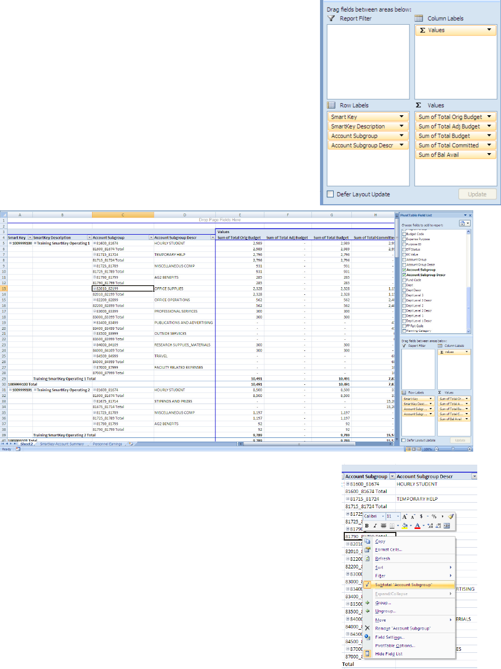
16. For the purpose of this training, we will arrange the PivotTable in the following manner:
17. Click each field from the upper section and drag it down to the appropriate field in the lower
section as shown on the right.
a. The Row Labels should be in the following order:
i. SmartKey
ii. SmartKey Description
iii. Account Subgroup
iv. Account Subgroup Descr
b. The Values should be in the following order
i. Total Orig Budget
ii. Total Adj Budget
iii. Total Budget
iv. Total Committed
v. Bal Avail
18. The PivotTable will now look like the image below:
19. By default, each Row Label is subtotaled. If you wish to remove
these subtotals, right click on the subtotal cell and deselect
“Subtotal Row Label.”
20. The subtotals can only be removed one at a time, per Row Label.
21. The PivotTable is now complete. You may format or resize the
columns as desired.
22. An example of the finished PivotTable is on Page 5.

5

6
23. Below is an example of a PivotTable run using the Personnel Earnings Report.
24. The criteria used are shown below.

7
Refreshing your Data
Once a PivotTable has been created, a user can easily update the data in the table without having to
reconstruct the entire PivotTable (or PivotTables). For example, a user can download month end report
data and simply refresh the PivotTable to update the data for the new month.
To update the PivotTable
1. Download new data.
2. Select all rows, excluding the header.
3. Copy selected rows.
4. Insert copied rows into PivotTable original data sheet.
5. Delete old data rows.
6. Right click on PivotTable and select “Refresh.”
7. The data shown in the PivotTable will now contain the new downloaded data.
